
InfluxQL functions
This page documents an earlier version of InfluxDB OSS. InfluxDB 3 Core is the latest stable version.
Aggregate, select, transform, and predict data with InfluxQL functions.
Content
Aggregations
COUNT()
Returns the number of non-null field values.
Syntax
SELECT COUNT( [ * | <field_key> | /<regular_expression>/ ] ) [INTO_clause] FROM_clause [WHERE_clause] [GROUP_BY_clause] [ORDER_BY_clause] [LIMIT_clause] [OFFSET_clause] [SLIMIT_clause] [SOFFSET_clause]Nested Syntax
SELECT COUNT(DISTINCT( [ * | <field_key> | /<regular_expression>/ ] )) [...]COUNT(field_key)
Returns the number of field values associated with the field key.
COUNT(/regular_expression/)
Returns the number of field values associated with each field key that matches the regular expression.
COUNT(*)
Returns the number of field values associated with each field key in the measurement.
COUNT() supports all field value data types.
InfluxQL supports nesting DISTINCT() with COUNT().
Examples
Count the field values associated with a field key
> SELECT COUNT("water_level") FROM "h2o_feet"

name: h2o_feet
time                   count
----                   -----
1970-01-01T00:00:00Z   15258
The query returns the number of non-null field values in the water_level field key in the h2o_feet measurement.
Count the field values associated with each field key in a measurement
> SELECT COUNT(*) FROM "h2o_feet"

name: h2o_feet
time                   count_level description   count_water_level
----                   -----------------------   -----------------
1970-01-01T00:00:00Z   15258                     15258
The query returns the number of non-null field values for each field key associated with the h2o_feet measurement.
The h2o_feet measurement has two field keys: level description and water_level.
Count the field values associated with each field key that matches a regular expression
> SELECT COUNT(/water/) FROM "h2o_feet"

name: h2o_feet
time                   count_water_level
----                   -----------------
1970-01-01T00:00:00Z   15258
The query returns the number of non-null field values for every field key that contains the word water in the h2o_feet measurement.
Count the field values associated with a field key and include several clauses
> SELECT COUNT("water_level") FROM "h2o_feet" WHERE time >= '2015-08-17T23:48:00Z' AND time <= '2015-08-18T00:54:00Z' GROUP BY time(12m),* fill(200) LIMIT 7 SLIMIT 1

name: h2o_feet
tags: location=coyote_creek
time                   count
----                   -----
2015-08-17T23:48:00Z   200
2015-08-18T00:00:00Z   2
2015-08-18T00:12:00Z   2
2015-08-18T00:24:00Z   2
2015-08-18T00:36:00Z   2
2015-08-18T00:48:00Z   2
The query returns the number of non-null field values in the water_level field key.
It covers the time range between 2015-08-17T23:48:00Z and 2015-08-18T00:54:00Z and groups results into 12-minute time intervals and per tag.
The query fills empty time intervals with 200 and limits the number of points and series returned to seven and one.
Count the distinct field values associated with a field key
> SELECT COUNT(DISTINCT("level description")) FROM "h2o_feet"

name: h2o_feet
time                   count
----                   -----
1970-01-01T00:00:00Z   4
The query returns the number of unique field values for the level description field key and the h2o_feet measurement.
Common Issues with COUNT()
COUNT() and fill()
Most InfluxQL functions report null values for time intervals with no data, and
fill(<fill_option>)
replaces that null value with the fill_option.
COUNT() reports 0 for time intervals with no data, and fill(<fill_option>) replaces any 0 values with the fill_option.
Example
The first query in the codeblock below does not include fill().
The last time interval has no data so the reported value for that time interval is zero.
The second query includes fill(800000); it replaces the zero in the last interval with 800000.
> SELECT COUNT("water_level") FROM "h2o_feet" WHERE time >= '2015-09-18T21:24:00Z' AND time <= '2015-09-18T21:54:00Z' GROUP BY time(12m)

name: h2o_feet
time                   count
----                   -----
2015-09-18T21:24:00Z   2
2015-09-18T21:36:00Z   2
2015-09-18T21:48:00Z   0

> SELECT COUNT("water_level") FROM "h2o_feet" WHERE time >= '2015-09-18T21:24:00Z' AND time <= '2015-09-18T21:54:00Z' GROUP BY time(12m) fill(800000)

name: h2o_feet
time                   count
----                   -----
2015-09-18T21:24:00Z   2
2015-09-18T21:36:00Z   2
2015-09-18T21:48:00Z   800000
DISTINCT()
Returns the list of unique field values.
Syntax
SELECT DISTINCT( [ <field_key> | /<regular_expression>/ ] ) FROM_clause [WHERE_clause] [GROUP_BY_clause] [ORDER_BY_clause] [LIMIT_clause] [OFFSET_clause] [SLIMIT_clause] [SOFFSET_clause]Nested Syntax
SELECT COUNT(DISTINCT( [ <field_key> | /<regular_expression>/ ] )) [...]DISTINCT(field_key)
Returns the unique field values associated with the field key.
DISTINCT() supports all field value data types.
InfluxQL supports nesting DISTINCT() with COUNT().
Examples
List the distinct field values associated with a field key
> SELECT DISTINCT("level description") FROM "h2o_feet"

name: h2o_feet
time                   distinct
----                   --------
1970-01-01T00:00:00Z   between 6 and 9 feet
1970-01-01T00:00:00Z   below 3 feet
1970-01-01T00:00:00Z   between 3 and 6 feet
1970-01-01T00:00:00Z   at or greater than 9 feet
The query returns a tabular list of the unique field values in the level description field key in the h2o_feet measurement.
List the distinct field values associated with each field key in a measurement
> SELECT DISTINCT(*) FROM "h2o_feet"

name: h2o_feet
time                   distinct_level description   distinct_water_level
----                   --------------------------   --------------------
1970-01-01T00:00:00Z   between 6 and 9 feet         8.12
1970-01-01T00:00:00Z   between 3 and 6 feet         8.005
1970-01-01T00:00:00Z   at or greater than 9 feet    7.887
1970-01-01T00:00:00Z   below 3 feet                 7.762
[...]
The query returns a tabular list of the unique field values for each field key in the h2o_feet measurement.
The h2o_feet measurement has two field keys: level description and water_level.
List the distinct field values associated with a field key and include several clauses
>  SELECT DISTINCT("level description") FROM "h2o_feet" WHERE time >= '2015-08-17T23:48:00Z' AND time <= '2015-08-18T00:54:00Z' GROUP BY time(12m),* SLIMIT 1

name: h2o_feet
tags: location=coyote_creek
time                   distinct
----                   --------
2015-08-18T00:00:00Z   between 6 and 9 feet
2015-08-18T00:12:00Z   between 6 and 9 feet
2015-08-18T00:24:00Z   between 6 and 9 feet
2015-08-18T00:36:00Z   between 6 and 9 feet
2015-08-18T00:48:00Z   between 6 and 9 feet
The query returns a tabular list of the unique field values in the level description field key.
It covers the time range between 2015-08-17T23:48:00Z and 2015-08-18T00:54:00Z and groups results into 12-minute time intervals and per tag.
The query also limits the number of series returned to one.
Count the distinct field values associated with a field key
> SELECT COUNT(DISTINCT("level description")) FROM "h2o_feet"

name: h2o_feet
time                   count
----                   -----
1970-01-01T00:00:00Z   4
The query returns the number of unique field values in the level description field key and the h2o_feet measurement.
Common Issues with DISTINCT()
DISTINCT() and the INTO clause
Using DISTINCT() with the INTO clause can cause InfluxDB to overwrite points in the destination measurement.
DISTINCT() often returns several results with the same timestamp; InfluxDB assumes points with the same series and timestamp are duplicate points and simply overwrites any duplicate point with the most recent point in the destination measurement.
Example
The first query in the codeblock below uses the DISTINCT() function and returns four results.
Notice that each result has the same timestamp.
The second query adds an INTO clause to the initial query and writes the query results to the distincts measurement.
The last query in the code block selects all the data in the distincts measurement.
The last query returns one point because the four initial results are duplicate points; they belong to the same series and have the same timestamp. When the system encounters duplicate points, it simply overwrites the previous point with the most recent point.
>  SELECT DISTINCT("level description") FROM "h2o_feet"

name: h2o_feet
time                   distinct
----                   --------
1970-01-01T00:00:00Z   below 3 feet
1970-01-01T00:00:00Z   between 6 and 9 feet
1970-01-01T00:00:00Z   between 3 and 6 feet
1970-01-01T00:00:00Z   at or greater than 9 feet

>  SELECT DISTINCT("level description") INTO "distincts" FROM "h2o_feet"

name: result
time                   written
----                   -------
1970-01-01T00:00:00Z   4

> SELECT * FROM "distincts"

name: distincts
time                   distinct
----                   --------
1970-01-01T00:00:00Z   at or greater than 9 feet
INTEGRAL()
Returns the area under the curve for subsequent field values.
Syntax
SELECT INTEGRAL( [ * | <field_key> | /<regular_expression>/ ] [ , <unit> ] ) [INTO_clause] FROM_clause [WHERE_clause] [GROUP_BY_clause] [ORDER_BY_clause] [LIMIT_clause] [OFFSET_clause] [SLIMIT_clause] [SOFFSET_clause]InfluxDB calculates the area under the curve for subsequent field values and converts those results into the summed area per unit.
The unit argument is an integer followed by a duration literal and it is optional.
If the query does not specify the unit, the unit defaults to one second (1s).
INTEGRAL(field_key)
Returns the area under the curve for subsequent field values associated with the field key.
INTEGRAL(/regular_expression/)
Returns the area under the curve for subsequent field values associated with each field key that matches the regular expression.
INTEGRAL(*)
Returns the average field value associated with each field key in the measurement.
INTEGRAL() does not support fill(). INTEGRAL() supports int64 and float64 field value data types.
Examples
Examples 1-5 use the following subsample of the NOAA_water_database data:
> SELECT "water_level" FROM "h2o_feet" WHERE "location" = 'santa_monica' AND time >= '2015-08-18T00:00:00Z' AND time <= '2015-08-18T00:30:00Z'

name: h2o_feet
time                   water_level
----                   -----------
2015-08-18T00:00:00Z   2.064
2015-08-18T00:06:00Z   2.116
2015-08-18T00:12:00Z   2.028
2015-08-18T00:18:00Z   2.126
2015-08-18T00:24:00Z   2.041
2015-08-18T00:30:00Z   2.051
Calculate the integral for the field values associated with a field key
> SELECT INTEGRAL("water_level") FROM "h2o_feet" WHERE "location" = 'santa_monica' AND time >= '2015-08-18T00:00:00Z' AND time <= '2015-08-18T00:30:00Z'

name: h2o_feet
time                 integral
----                 --------
1970-01-01T00:00:00Z 3732.66
The query returns the area under the curve (in seconds) for the field values associated with the water_level field key and in the h2o_feet measurement.
Calculate the integral for the field values associated with a field key and specify the unit option
> SELECT INTEGRAL("water_level",1m) FROM "h2o_feet" WHERE "location" = 'santa_monica' AND time >= '2015-08-18T00:00:00Z' AND time <= '2015-08-18T00:30:00Z'

name: h2o_feet
time                 integral
----                 --------
1970-01-01T00:00:00Z 62.211
The query returns the area under the curve (in minutes) for the field values associated with the water_level field key and in the h2o_feet measurement.
Calculate the integral for the field values associated with each field key in a measurement and specify the unit option
> SELECT INTEGRAL(*,1m) FROM "h2o_feet" WHERE "location" = 'santa_monica' AND time >= '2015-08-18T00:00:00Z' AND time <= '2015-08-18T00:30:00Z'

name: h2o_feet
time                 integral_water_level
----                 --------------------
1970-01-01T00:00:00Z 62.211
The query returns the area under the curve (in minutes) for the field values associated with each field key that stores numerical values in the h2o_feet measurement.
The h2o_feet measurement has on numerical field: water_level.
Calculate the integral for the field values associated with each field key that matches a regular expression and specify the unit option
> SELECT INTEGRAL(/water/,1m) FROM "h2o_feet" WHERE "location" = 'santa_monica' AND time >= '2015-08-18T00:00:00Z' AND time <= '2015-08-18T00:30:00Z'

name: h2o_feet
time                 integral_water_level
----                 --------------------
1970-01-01T00:00:00Z 62.211
The query returns the area under the curve (in minutes) for the field values associated with each field key that stores numerical values includes the word water in the h2o_feet measurement.
Calculate the integral for the field values associated with a field key and include several clauses
> SELECT INTEGRAL("water_level",1m) FROM "h2o_feet" WHERE "location" = 'santa_monica' AND time >= '2015-08-18T00:00:00Z' AND time <= '2015-08-18T00:30:00Z' GROUP BY time(12m) LIMIT 1

name: h2o_feet
time                 integral
----                 --------
2015-08-18T00:00:00Z 24.972
The query returns the area under the curve (in minutes) for the field values associated with the water_level field key and in the h2o_feet measurement.
It covers the time range between 2015-08-18T00:00:00Z and 2015-08-18T00:30:00Z, groups results into 12-minute intervals, and limits the number of results returned to one.
MEAN()
Returns the arithmetic mean (average) of field values.
Syntax
SELECT MEAN( [ * | <field_key> | /<regular_expression>/ ] ) [INTO_clause] FROM_clause [WHERE_clause] [GROUP_BY_clause] [ORDER_BY_clause] [LIMIT_clause] [OFFSET_clause] [SLIMIT_clause] [SOFFSET_clause]MEAN(field_key)
Returns the average field value associated with the field key.
MEAN(/regular_expression/)
Returns the average field value associated with each field key that matches the regular expression.
MEAN(*)
Returns the average field value associated with each field key in the measurement.
MEAN() supports int64 and float64 field value data types.
Examples
Calculate the mean field value associated with a field key
> SELECT MEAN("water_level") FROM "h2o_feet"

name: h2o_feet
time                   mean
----                   ----
1970-01-01T00:00:00Z   4.442107025822522
The query returns the average field value in the water_level field key in the h2o_feet measurement.
Calculate the mean field value associated with each field key in a measurement
> SELECT MEAN(*) FROM "h2o_feet"

name: h2o_feet
time                   mean_water_level
----                   ----------------
1970-01-01T00:00:00Z   4.442107025822522
The query returns the average field value for every field key that stores numerical values in the h2o_feet measurement.
The h2o_feet measurement has one numerical field: water_level.
Calculate the mean field value associated with each field key that matches a regular expression
> SELECT MEAN(/water/) FROM "h2o_feet"

name: h2o_feet
time                   mean_water_level
----                   ----------------
1970-01-01T00:00:00Z   4.442107025822523
The query returns the average field value for each field key that stores numerical values and includes the word water in the h2o_feet measurement.
Calculate the mean field value associated with a field key and include several clauses
> SELECT MEAN("water_level") FROM "h2o_feet" WHERE time >= '2015-08-17T23:48:00Z' AND time <= '2015-08-18T00:54:00Z' GROUP BY time(12m),* fill(9.01) LIMIT 7 SLIMIT 1

name: h2o_feet
tags: location=coyote_creek
time                   mean
----                   ----
2015-08-17T23:48:00Z   9.01
2015-08-18T00:00:00Z   8.0625
2015-08-18T00:12:00Z   7.8245
2015-08-18T00:24:00Z   7.5675
2015-08-18T00:36:00Z   7.303
2015-08-18T00:48:00Z   7.046
The query returns the average of the values in the water_level field key.
It covers the time range between 2015-08-17T23:48:00Z and 2015-08-18T00:54:00Z and groups results into 12-minute time intervals and per tag.
The query fills empty time intervals with 9.01 and limits the number of points and series returned to seven and one.
MEDIAN()
Returns the middle value from a sorted list of field values.
Syntax
SELECT MEDIAN( [ * | <field_key> | /<regular_expression>/ ] ) [INTO_clause] FROM_clause [WHERE_clause] [GROUP_BY_clause] [ORDER_BY_clause] [LIMIT_clause] [OFFSET_clause] [SLIMIT_clause] [SOFFSET_clause]MEDIAN(field_key)
Returns the middle field value associated with the field key.
MEDIAN(/regular_expression/)
Returns the middle field value associated with each field key that matches the regular expression.
MEDIAN(*)
Returns the middle field value associated with each field key in the measurement.
MEDIAN() supports int64 and float64 field value data types.
Note:
MEDIAN()is nearly equivalent toPERCENTILE(field_key, 50), exceptMEDIAN()returns the average of the two middle field values if the field contains an even number of values.
Examples
Calculate the median field value associated with a field key
> SELECT MEDIAN("water_level") FROM "h2o_feet"

name: h2o_feet
time                   median
----                   ------
1970-01-01T00:00:00Z   4.124
The query returns the middle field value in the water_level field key and in the h2o_feet measurement.
Calculate the median field value associated with each field key in a measurement
> SELECT MEDIAN(*) FROM "h2o_feet"

name: h2o_feet
time                   median_water_level
----                   ------------------
1970-01-01T00:00:00Z   4.124
The query returns the middle field value for every field key that stores numerical values in the h2o_feet measurement.
The h2o_feet measurement has one numerical field: water_level.
Calculate the median field value associated with each field key that matches a regular expression
> SELECT MEDIAN(/water/) FROM "h2o_feet"

name: h2o_feet
time                   median_water_level
----                   ------------------
1970-01-01T00:00:00Z   4.124
The query returns the middle field value for every field key that stores numerical values and includes the word water in the h2o_feet measurement.
Calculate the median field value associated with a field key and include several clauses
> SELECT MEDIAN("water_level") FROM "h2o_feet" WHERE time >= '2015-08-17T23:48:00Z' AND time <= '2015-08-18T00:54:00Z' GROUP BY time(12m),* fill(700) LIMIT 7 SLIMIT 1 SOFFSET 1

name: h2o_feet
tags: location=santa_monica
time                   median
----                   ------
2015-08-17T23:48:00Z   700
2015-08-18T00:00:00Z   2.09
2015-08-18T00:12:00Z   2.077
2015-08-18T00:24:00Z   2.0460000000000003
2015-08-18T00:36:00Z   2.0620000000000003
2015-08-18T00:48:00Z   700
The query returns the middle field value in the water_level field key.
It covers the time range between 2015-08-17T23:48:00Z and 2015-08-18T00:54:00Z and groups results into 12-minute time intervals and per tag.
The query fills empty time intervals with 700 , limits the number of points and series returned to seven and one, and offsets the series returned by one.
MODE()
Returns the most frequent value in a list of field values.
Syntax
SELECT MODE( [ * | <field_key> | /<regular_expression>/ ] ) [INTO_clause] FROM_clause [WHERE_clause] [GROUP_BY_clause] [ORDER_BY_clause] [LIMIT_clause] [OFFSET_clause] [SLIMIT_clause] [SOFFSET_clause]MODE(field_key)
Returns the most frequent field value associated with the field key.
MODE(/regular_expression/)
Returns the most frequent field value associated with each field key that matches the regular expression.
MODE(*)
Returns the most frequent field value associated with each field key in the measurement.
MODE() supports all field value data types.
Note:
MODE()returns the field value with the earliest timestamp if there’s a tie between two or more values for the maximum number of occurrences.
Examples
Calculate the mode field value associated with a field key
> SELECT MODE("level description") FROM "h2o_feet"

name: h2o_feet
time                   mode
----                   ----
1970-01-01T00:00:00Z   between 3 and 6 feet
The query returns the most frequent field value in the level description field key and in the h2o_feet measurement.
Calculate the mode field value associated with each field key in a measurement
> SELECT MODE(*) FROM "h2o_feet"

name: h2o_feet
time                   mode_level description   mode_water_level
----                   ----------------------   ----------------
1970-01-01T00:00:00Z   between 3 and 6 feet     2.69
The query returns the most frequent field value for every field key in the h2o_feet measurement.
The h2o_feet measurement has two field keys: level description and water_level.
Calculate the mode field value associated with each field key that matches a regular expression
> SELECT MODE(/water/) FROM "h2o_feet"

name: h2o_feet
time                   mode_water_level
----                   ----------------
1970-01-01T00:00:00Z   2.69
The query returns the most frequent field value for every field key that includes the word /water/ in the h2o_feet measurement.
Calculate the mode field value associated with a field key and include several clauses
> SELECT MODE("level description") FROM "h2o_feet" WHERE time >= '2015-08-17T23:48:00Z' AND time <= '2015-08-18T00:54:00Z' GROUP BY time(12m),* LIMIT 3 SLIMIT 1 SOFFSET 1

name: h2o_feet
tags: location=santa_monica
time                   mode
----                   ----
2015-08-17T23:48:00Z
2015-08-18T00:00:00Z   below 3 feet
2015-08-18T00:12:00Z   below 3 feet
The query returns the mode of the values associated with the water_level field key.
It covers the time range between 2015-08-17T23:48:00Z and 2015-08-18T00:54:00Z and groups results into 12-minute time intervals and per tag.
The query limits the number of points and series returned to three and one, and it offsets the series returned by one.
SPREAD()
Returns the difference between the minimum and maximum field values.
Syntax
SELECT SPREAD( [ * | <field_key> | /<regular_expression>/ ] ) [INTO_clause] FROM_clause [WHERE_clause] [GROUP_BY_clause] [ORDER_BY_clause] [LIMIT_clause] [OFFSET_clause] [SLIMIT_clause] [SOFFSET_clause]SPREAD(field_key)
Returns the difference between the minimum and maximum field values associated with the field key.
SPREAD(/regular_expression/)
Returns the difference between the minimum and maximum field values associated with each field key that matches the regular expression.
SPREAD(*)
Returns the difference between the minimum and maximum field values associated with each field key in the measurement.
SPREAD() supports int64 and float64 field value data types.
Examples
Calculate the spread for the field values associated with a field key
> SELECT SPREAD("water_level") FROM "h2o_feet"

name: h2o_feet
time                   spread
----                   ------
1970-01-01T00:00:00Z   10.574
The query returns the difference between the minimum and maximum field values in the water_level field key and in the h2o_feet measurement.
Calculate the spread for the field values associated with each field key in a measurement
> SELECT SPREAD(*) FROM "h2o_feet"

name: h2o_feet
time                   spread_water_level
----                   ------------------
1970-01-01T00:00:00Z   10.574
The query returns the difference between the minimum and maximum field values for every field key that stores numerical values in the h2o_feet measurement.
The h2o_feet measurement has one numerical field: water_level.
Calculate the spread for the field values associated with each field key that matches a regular expression
> SELECT SPREAD(/water/) FROM "h2o_feet"

name: h2o_feet
time                   spread_water_level
----                   ------------------
1970-01-01T00:00:00Z   10.574
The query returns the difference between the minimum and maximum field values for every field key that stores numerical values and includes the word water in the h2o_feet measurement.
Calculate the spread for the field values associated with a field key and include several clauses
> SELECT SPREAD("water_level") FROM "h2o_feet" WHERE time >= '2015-08-17T23:48:00Z' AND time <= '2015-08-18T00:54:00Z' GROUP BY time(12m),* fill(18) LIMIT 3 SLIMIT 1 SOFFSET 1

name: h2o_feet
tags: location=santa_monica
time                   spread
----                   ------
2015-08-17T23:48:00Z   18
2015-08-18T00:00:00Z   0.052000000000000046
2015-08-18T00:12:00Z   0.09799999999999986
The query returns the difference between the minimum and maximum field values in the water_level field key.
It covers the time range between 2015-08-17T23:48:00Z and 2015-08-18T00:54:00Z and groups results into 12-minute time intervals and per tag.
The query fills empty time intervals with 18, limits the number of points and series returned to three and one, and offsets the series returned by one.
STDDEV()
Returns the standard deviation of field values.
Syntax
SELECT STDDEV( [ * | <field_key> | /<regular_expression>/ ] ) [INTO_clause] FROM_clause [WHERE_clause] [GROUP_BY_clause] [ORDER_BY_clause] [LIMIT_clause] [OFFSET_clause] [SLIMIT_clause] [SOFFSET_clause]STDDEV(field_key)
Returns the standard deviation of field values associated with the field key.
STDDEV(/regular_expression/)
Returns the standard deviation of field values associated with each field key that matches the regular expression.
STDDEV(*)
Returns the standard deviation of field values associated with each field key in the measurement.
STDDEV() supports int64 and float64 field value data types.
Examples
Calculate the standard deviation for the field values associated with a field key
> SELECT STDDEV("water_level") FROM "h2o_feet"

name: h2o_feet
time                   stddev
----                   ------
1970-01-01T00:00:00Z   2.279144584196141
The query returns the standard deviation of the field values in the water_level field key and in the h2o_feet measurement.
Calculate the standard deviation for the field values associated with each field key in a measurement
> SELECT STDDEV(*) FROM "h2o_feet"

name: h2o_feet
time                   stddev_water_level
----                   ------------------
1970-01-01T00:00:00Z   2.279144584196141
The query returns the standard deviation of the field values for each field key that stores numerical values in the h2o_feet measurement.
The h2o_feet measurement has one numerical field: water_level.
Calculate the standard deviation for the field values associated with each field key that matches a regular expression
> SELECT STDDEV(/water/) FROM "h2o_feet"

name: h2o_feet
time                   stddev_water_level
----                   ------------------
1970-01-01T00:00:00Z   2.279144584196141
The query returns the standard deviation of the field values for each field key that stores numerical values and includes the word water in the h2o_feet measurement.
Calculate the standard deviation for the field values associated with a field key and include several clauses
> SELECT STDDEV("water_level") FROM "h2o_feet" WHERE time >= '2015-08-17T23:48:00Z' AND time <= '2015-08-18T00:54:00Z' GROUP BY time(12m),* fill(18000) LIMIT 2 SLIMIT 1 SOFFSET 1

name: h2o_feet
tags: location=santa_monica
time                   stddev
----                   ------
2015-08-17T23:48:00Z   18000
2015-08-18T00:00:00Z   0.03676955262170051
The query returns the standard deviation of the field values in the water_level field key.
It covers the time range between 2015-08-17T23:48:00Z and 2015-08-18T00:54:00Z and groups results into 12-minute time intervals and per tag.
The query fills empty time intervals with 18000, limits the number of points and series returned to two and one, and offsets the series returned by one.
SUM()
Returns the sum of field values.
Syntax
SELECT SUM( [ * | <field_key> | /<regular_expression>/ ] ) [INTO_clause] FROM_clause [WHERE_clause] [GROUP_BY_clause] [ORDER_BY_clause] [LIMIT_clause] [OFFSET_clause] [SLIMIT_clause] [SOFFSET_clause]SUM(field_key)
Returns the sum of field values associated with the field key.
SUM(/regular_expression/)
Returns the sum of field values associated with each field key that matches the regular expression.
SUM(*)
Returns the sums of field values associated with each field key in the measurement.
SUM() supports int64 and float64 field value data types.
Examples
Calculate the sum of the field values associated with a field key
> SELECT SUM("water_level") FROM "h2o_feet"

name: h2o_feet
time                   sum
----                   ---
1970-01-01T00:00:00Z   67777.66900000004
The query returns the summed total of the field values in the water_level field key and in the h2o_feet measurement.
Calculate the sum of the field values associated with each field key in a measurement
> SELECT SUM(*) FROM "h2o_feet"

name: h2o_feet
time                   sum_water_level
----                   ---------------
1970-01-01T00:00:00Z   67777.66900000004
The query returns the summed total of the field values for each field key that stores numerical values in the h2o_feet measurement.
The h2o_feet measurement has one numerical field: water_level.
Calculate the sum of the field values associated with each field key that matches a regular expression
> SELECT SUM(/water/) FROM "h2o_feet"

name: h2o_feet
time                   sum_water_level
----                   ---------------
1970-01-01T00:00:00Z   67777.66900000004
The query returns the summed total of the field values for each field key that stores numerical values and includes the word water in the h2o_feet measurement.
Calculate the sum of the field values associated with a field key and include several clauses
> SELECT SUM("water_level") FROM "h2o_feet" WHERE time >= '2015-08-17T23:48:00Z' AND time <= '2015-08-18T00:54:00Z' GROUP BY time(12m),* fill(18000) LIMIT 4 SLIMIT 1

name: h2o_feet
tags: location=coyote_creek
time                   sum
----                   ---
2015-08-17T23:48:00Z   18000
2015-08-18T00:00:00Z   16.125
2015-08-18T00:12:00Z   15.649
2015-08-18T00:24:00Z   15.135
The query returns the summed total of the field values in the water_level field key.
It covers the time range between 2015-08-17T23:48:00Z and 2015-08-18T00:54:00Z and groups results into 12-minute time intervals and per tag. The query fills empty time intervals with 18000, and it limits the number of points and series returned to four and one.
Selectors
BOTTOM()
Returns the smallest N field values.
Syntax
SELECT BOTTOM(<field_key>[,<tag_key(s)>],<N> )[,<tag_key(s)>|<field_key(s)>] [INTO_clause] FROM_clause [WHERE_clause] [GROUP_BY_clause] [ORDER_BY_clause] [LIMIT_clause] [OFFSET_clause] [SLIMIT_clause] [SOFFSET_clause]BOTTOM(field_key,N)
Returns the smallest N field values associated with the field key.
BOTTOM(field_key,tag_key(s),N)
Returns the smallest field value for N tag values of the tag key.
BOTTOM(field_key,N),tag_key(s),field_key(s)
Returns the smallest N field values associated with the field key in the parentheses and the relevant tag and/or field.
BOTTOM() supports int64 and float64 field value data types.
Notes:
BOTTOM()returns the field value with the earliest timestamp if there’s a tie between two or more values for the smallest value.BOTTOM()differs from other InfluxQL functions when combined with anINTOclause. See the Common Issues section for more information.
Examples
Select the bottom three field values associated with a field key
> SELECT BOTTOM("water_level",3) FROM "h2o_feet"

name: h2o_feet
time                   bottom
----                   ------
2015-08-29T14:30:00Z   -0.61
2015-08-29T14:36:00Z   -0.591
2015-08-30T15:18:00Z   -0.594
The query returns the smallest three field values in the water_level field key and in the h2o_feet measurement.
Select the bottom field value associated with a field key for two tags
> SELECT BOTTOM("water_level","location",2) FROM "h2o_feet"

name: h2o_feet
time                   bottom   location
----                   ------   --------
2015-08-29T10:36:00Z   -0.243   santa_monica
2015-08-29T14:30:00Z   -0.61    coyote_creek
The query returns the smallest field values in the water_level field key for two tag values associated with the location tag key.
Select the bottom four field values associated with a field key and the relevant tags and fields
> SELECT BOTTOM("water_level",4),"location","level description" FROM "h2o_feet"

name: h2o_feet
time                  bottom  location      level description
----                  ------  --------      -----------------
2015-08-29T14:24:00Z  -0.587  coyote_creek  below 3 feet
2015-08-29T14:30:00Z  -0.61   coyote_creek  below 3 feet
2015-08-29T14:36:00Z  -0.591  coyote_creek  below 3 feet
2015-08-30T15:18:00Z  -0.594  coyote_creek  below 3 feet
The query returns the smallest four field values in the water_level field key and the relevant values of the location tag key and the level description field key.
Select the bottom three field values associated with a field key and include several clauses
> SELECT BOTTOM("water_level",3),"location" FROM "h2o_feet" WHERE time >= '2015-08-18T00:00:00Z' AND time <= '2015-08-18T00:54:00Z' GROUP BY time(24m) ORDER BY time DESC

name: h2o_feet
time                  bottom  location
----                  ------  --------
2015-08-18T00:48:00Z  1.991   santa_monica
2015-08-18T00:54:00Z  2.054   santa_monica
2015-08-18T00:54:00Z  6.982   coyote_creek
2015-08-18T00:24:00Z  2.041   santa_monica
2015-08-18T00:30:00Z  2.051   santa_monica
2015-08-18T00:42:00Z  2.057   santa_monica
2015-08-18T00:00:00Z  2.064   santa_monica
2015-08-18T00:06:00Z  2.116   santa_monica
2015-08-18T00:12:00Z  2.028   santa_monica
The query returns the smallest three values in the water_level field key for each 24-minute interval between 2015-08-18T00:00:00Z and 2015-08-18T00:54:00Z.
It also returns results in descending timestamp order.
Notice that the GROUP BY time() clause does not override the points’ original timestamps. See Issue 1 in the section below for a more detailed explanation of that behavior.
Common Issues with BOTTOM()
BOTTOM() with a GROUP BY time() clause
Queries with BOTTOM() and a GROUP BY time() clause return the specified
number of points per GROUP BY time() interval.
For
most GROUP BY time() queries,
the returned timestamps mark the start of the GROUP BY time() interval.
GROUP BY time() queries with the BOTTOM() function behave differently;
they maintain the timestamp of the original data point.
Example
The query below returns two points per 18-minute
GROUP BY time() interval.
Notice that the returned timestamps are the points’ original timestamps; they
are not forced to match the start of the GROUP BY time() intervals.
> SELECT BOTTOM("water_level",2) FROM "h2o_feet" WHERE time >= '2015-08-18T00:00:00Z' AND time <= '2015-08-18T00:30:00Z' AND "location" = 'santa_monica' GROUP BY time(18m)

name: h2o_feet
time                   bottom
----                   ------
                           __
2015-08-18T00:00:00Z  2.064 |
2015-08-18T00:12:00Z  2.028 | <------- Smallest points for the first time interval
                           --
                           __
2015-08-18T00:24:00Z  2.041 |
2015-08-18T00:30:00Z  2.051 | <------- Smallest points for the second time interval                      --
BOTTOM() and a tag key with fewer than N tag values
Queries with the syntax SELECT BOTTOM(<field_key>,<tag_key>,<N>) can return fewer points than expected.
If the tag key has X tag values, the query specifies N values, and X is smaller than N, then the query returns X points.
Example
The query below asks for the smallest field values of water_level for three tag values of the location tag key.
Because the location tag key has two tag values (santa_monica and coyote_creek), the query returns two points instead of three.
> SELECT BOTTOM("water_level","location",3) FROM "h2o_feet"

name: h2o_feet
time                   bottom   location
----                   ------   --------
2015-08-29T10:36:00Z   -0.243   santa_monica
2015-08-29T14:30:00Z   -0.61    coyote_creek
BOTTOM(), tags, and the INTO clause
When combined with an INTO clause and no GROUP BY tag clause, most InfluxQL functions convert any tags in the initial data to fields in the newly written data.
This behavior also applies to the BOTTOM() function unless BOTTOM() includes a tag key as an argument: BOTTOM(field_key,tag_key(s),N).
In those cases, the system preserves the specified tag as a tag in the newly written data.
Example
The first query in the codeblock below returns the smallest field values in the water_level field key for two tag values associated with the location tag key.
It also writes those results to the bottom_water_levels measurement.
The second query shows that InfluxDB preserved the location tag as a tag in the bottom_water_levels measurement.
> SELECT BOTTOM("water_level","location",2) INTO "bottom_water_levels" FROM "h2o_feet"

name: result
time                 written
----                 -------
1970-01-01T00:00:00Z 2

> SHOW TAG KEYS FROM "bottom_water_levels"

name: bottom_water_levels
tagKey
------
location
FIRST()
Returns the field value with the oldest timestamp.
Syntax
SELECT FIRST(<field_key>)[,<tag_key(s)>|<field_key(s)>] [INTO_clause] FROM_clause [WHERE_clause] [GROUP_BY_clause] [ORDER_BY_clause] [LIMIT_clause] [OFFSET_clause] [SLIMIT_clause] [SOFFSET_clause]FIRST(field_key)
Returns the oldest field value (determined by timestamp) associated with the field key.
FIRST(/regular_expression/)
Returns the oldest field value (determined by timestamp) associated with each field key that matches the regular expression.
FIRST(*)
Returns the oldest field value (determined by timestamp) associated with each field key in the measurement.
FIRST(field_key),tag_key(s),field_key(s)
Returns the oldest field value (determined by timestamp) associated with the field key in the parentheses and the relevant tag and/or field.
FIRST() supports all field value data types.
Examples
Select the first field value associated with a field key
> SELECT FIRST("level description") FROM "h2o_feet"

name: h2o_feet
time                   first
----                   -----
2015-08-18T00:00:00Z   between 6 and 9 feet
The query returns the oldest field value (determined by timestamp) associated with the level description field key and in the h2o_feet measurement.
Select the first field value associated with each field key in a measurement
> SELECT FIRST(*) FROM "h2o_feet"

name: h2o_feet
time                   first_level description   first_water_level
----                   -----------------------   -----------------
1970-01-01T00:00:00Z   between 6 and 9 feet      8.12
The query returns the oldest field value (determined by timestamp) for each field key in the h2o_feet measurement.
The h2o_feet measurement has two field keys: level description and water_level.
Select the first field value associated with each field key that matches a regular expression
> SELECT FIRST(/level/) FROM "h2o_feet"

name: h2o_feet
time                   first_level description   first_water_level
----                   -----------------------   -----------------
1970-01-01T00:00:00Z   between 6 and 9 feet      8.12
The query returns the oldest field value for each field key that includes the word level in the h2o_feet measurement.
Select the first value associated with a field key and the relevant tags and fields
> SELECT FIRST("level description"),"location","water_level" FROM "h2o_feet"

name: h2o_feet
time                  first                 location      water_level
----                  -----                 --------      -----------
2015-08-18T00:00:00Z  between 6 and 9 feet  coyote_creek  8.12
The query returns the oldest field value (determined by timestamp) in the level description field key and the relevant values of the location tag key and the water_level field key.
Select the first field value associated with a field key and include several clauses
> SELECT FIRST("water_level") FROM "h2o_feet" WHERE time >= '2015-08-17T23:48:00Z' AND time <= '2015-08-18T00:54:00Z' GROUP BY time(12m),* fill(9.01) LIMIT 4 SLIMIT 1

name: h2o_feet
tags: location=coyote_creek
time                   first
----                   -----
2015-08-17T23:48:00Z   9.01
2015-08-18T00:00:00Z   8.12
2015-08-18T00:12:00Z   7.887
2015-08-18T00:24:00Z   7.635
The query returns the oldest field value (determined by timestamp) in the water_level field key.
It covers the time range between 2015-08-17T23:48:00Z and 2015-08-18T00:54:00Z and groups results into 12-minute time intervals and per tag.
The query fills empty time intervals with 9.01, and it limits the number of points and series returned to four and one.
Notice that the GROUP BY time() clause overrides the points’ original timestamps.
The timestamps in the results indicate the the start of each 12-minute time interval;
the first point in the results covers the time interval between 2015-08-17T23:48:00Z and just before 2015-08-18T00:00:00Z and the last point in the results covers the time interval between 2015-08-18T00:24:00Z and just before 2015-08-18T00:36:00Z.
LAST()
Returns the field value with the most recent timestamp.
Syntax
SELECT LAST(<field_key>)[,<tag_key(s)>|<field_keys(s)>] [INTO_clause] FROM_clause [WHERE_clause] [GROUP_BY_clause] [ORDER_BY_clause] [LIMIT_clause] [OFFSET_clause] [SLIMIT_clause] [SOFFSET_clause]LAST(field_key)
Returns the newest field value (determined by timestamp) associated with the field key.
LAST(/regular_expression/)
Returns the newest field value (determined by timestamp) associated with each field key that matches the regular expression.
LAST(*)
Returns the newest field value (determined by timestamp) associated with each field key in the measurement.
LAST(field_key),tag_key(s),field_key(s)
Returns the newest field value (determined by timestamp) associated with the field key in the parentheses and the relevant tag and/or field.
LAST() supports all field value data types.
Examples
Select the last field values associated with a field key
> SELECT LAST("level description") FROM "h2o_feet"

name: h2o_feet
time                   last
----                   ----
2015-09-18T21:42:00Z   between 3 and 6 feet
The query returns the newest field value (determined by timestamp) associated with the level description field key and in the h2o_feet measurement.
Select the last field values associated with each field key in a measurement
> SELECT LAST(*) FROM "h2o_feet"

name: h2o_feet
time                   last_level description   last_water_level
----                   -----------------------   -----------------
1970-01-01T00:00:00Z   between 3 and 6 feet      4.938
The query returns the newest field value (determined by timestamp) for each field key in the h2o_feet measurement.
The h2o_feet measurement has two field keys: level description and water_level.
Select the last field value associated with each field key that matches a regular expression
> SELECT LAST(/level/) FROM "h2o_feet"

name: h2o_feet
time                   last_level description   last_water_level
----                   -----------------------   -----------------
1970-01-01T00:00:00Z   between 3 and 6 feet      4.938
The query returns the newest field value for each field key that includes the word level in the h2o_feet measurement.
Select the last field value associated with a field key and the relevant tags and fields
> SELECT LAST("level description"),"location","water_level" FROM "h2o_feet"

name: h2o_feet
time                  last                  location      water_level
----                  ----                  --------      -----------
2015-09-18T21:42:00Z  between 3 and 6 feet  santa_monica  4.938
The query returns the newest field value (determined by timestamp) in the level description field key and the relevant values of the location tag key and the water_level field key.
Select the last field value associated with a field key and include several clauses
> SELECT LAST("water_level") FROM "h2o_feet" WHERE time >= '2015-08-17T23:48:00Z' AND time <= '2015-08-18T00:54:00Z' GROUP BY time(12m),* fill(9.01) LIMIT 4 SLIMIT 1

name: h2o_feet
tags: location=coyote_creek
time                   last
----                   ----
2015-08-17T23:48:00Z   9.01
2015-08-18T00:00:00Z   8.005
2015-08-18T00:12:00Z   7.762
2015-08-18T00:24:00Z   7.5
The query returns the newest field value (determined by timestamp) in the water_level field key.
It covers the time range between 2015-08-17T23:48:00Z and 2015-08-18T00:54:00Z and groups results into 12-minute time intervals and per tag.
The query fills empty time intervals with 9.01, and it limits the number of points and series returned to four and one.
Notice that the GROUP BY time() clause overrides the points’ original timestamps.
The timestamps in the results indicate the the start of each 12-minute time interval;
the first point in the results covers the time interval between 2015-08-17T23:48:00Z and just before 2015-08-18T00:00:00Z and the last point in the results covers the time interval between 2015-08-18T00:24:00Z and just before 2015-08-18T00:36:00Z.
MAX()
Returns the greatest field value.
Syntax
SELECT MAX(<field_key>)[,<tag_key(s)>|<field__key(s)>] [INTO_clause] FROM_clause [WHERE_clause] [GROUP_BY_clause] [ORDER_BY_clause] [LIMIT_clause] [OFFSET_clause] [SLIMIT_clause] [SOFFSET_clause]MAX(field_key)
Returns the greatest field value associated with the field key.
MAX(/regular_expression/)
Returns the greatest field value associated with each field key that matches the regular expression.
MAX(*)
Returns the greatest field value associated with each field key in the measurement.
MAX(field_key),tag_key(s),field_key(s)
Returns the greatest field value associated with the field key in the parentheses and the relevant tag and/or field.
MAX() supports int64 and float64 field value data types.
Examples
Select the maximum field value associated with a field key
> SELECT MAX("water_level") FROM "h2o_feet"

name: h2o_feet
time                   max
----                   ---
2015-08-29T07:24:00Z   9.964
The query returns the greatest field value in the water_level field key and in the h2o_feet measurement.
Select the maximum field value associated with each field key in a measurement
> SELECT MAX(*) FROM "h2o_feet"

name: h2o_feet
time                   max_water_level
----                   ---------------
2015-08-29T07:24:00Z   9.964
The query returns the greatest field value for each field key that stores numerical values in the h2o_feet measurement.
The h2o_feet measurement has one numerical field: water_level.
Select the maximum field value associated with each field key that matches a regular expression
> SELECT MAX(/level/) FROM "h2o_feet"

name: h2o_feet
time                   max_water_level
----                   ---------------
2015-08-29T07:24:00Z   9.964
The query returns the greatest field value for each field key that stores numerical values and includes the word water in the h2o_feet measurement.
Select the maximum field value associated with a field key and the relevant tags and fields
> SELECT MAX("water_level"),"location","level description" FROM "h2o_feet"

name: h2o_feet
time                  max    location      level description
----                  ---    --------      -----------------
2015-08-29T07:24:00Z  9.964  coyote_creek  at or greater than 9 feet
The query returns the greatest field value in the water_level field key and the relevant values of the location tag key and the level description field key.
Select the maximum field value associated with a field key and include several clauses
> SELECT MAX("water_level") FROM "h2o_feet" WHERE time >= '2015-08-17T23:48:00Z' AND time <= '2015-08-18T00:54:00Z' GROUP BY time(12m),* fill(9.01) LIMIT 4 SLIMIT 1

name: h2o_feet
tags: location=coyote_creek
time                   max
----                   ---
2015-08-17T23:48:00Z   9.01
2015-08-18T00:00:00Z   8.12
2015-08-18T00:12:00Z   7.887
2015-08-18T00:24:00Z   7.635
The query returns the greatest field value in the water_level field key.
It covers the time range between 2015-08-17T23:48:00Z and 2015-08-18T00:54:00Z and groups results in to 12-minute time intervals and per tag.
The query fills empty time intervals with 9.01, and it limits the number of points and series returned to four and one.
Notice that the GROUP BY time() clause overrides the points’ original timestamps.
The timestamps in the results indicate the the start of each 12-minute time interval;
the first point in the results covers the time interval between 2015-08-17T23:48:00Z and just before 2015-08-18T00:00:00Z and the last point in the results covers the time interval between 2015-08-18T00:24:00Z and just before 2015-08-18T00:36:00Z.
MIN()
Returns the lowest field value.
Syntax
SELECT MIN(<field_key>)[,<tag_key(s)>|<field_key(s)>] [INTO_clause] FROM_clause [WHERE_clause] [GROUP_BY_clause] [ORDER_BY_clause] [LIMIT_clause] [OFFSET_clause] [SLIMIT_clause] [SOFFSET_clause]MIN(field_key)
Returns the lowest field value associated with the field key.
MIN(/regular_expression/)
Returns the lowest field value associated with each field key that matches the regular expression.
MIN(*)
Returns the lowest field value associated with each field key in the measurement.
MIN(field_key),tag_key(s),field_key(s)
Returns the lowest field value associated with the field key in the parentheses and the relevant tag and/or field.
MIN() supports int64 and float64 field value data types.
Examples
Select the minimum field value associated with a field key
> SELECT MIN("water_level") FROM "h2o_feet"

name: h2o_feet
time                   min
----                   ---
2015-08-29T14:30:00Z   -0.61
The query returns the lowest field value in the water_level field key and in the h2o_feet measurement.
Select the minimum field value associated with each field key in a measurement
> SELECT MIN(*) FROM "h2o_feet"

name: h2o_feet
time                   min_water_level
----                   ---------------
2015-08-29T14:30:00Z   -0.61
The query returns the lowest field value for each field key that stores numerical values in the h2o_feet measurement.
The h2o_feet measurement has one numerical field: water_level.
Select the minimum field value associated with each field key that matches a regular expression
> SELECT MIN(/level/) FROM "h2o_feet"

name: h2o_feet
time                   min_water_level
----                   ---------------
2015-08-29T14:30:00Z   -0.61
The query returns the lowest field value for each field key that stores numerical values and includes the word water in the h2o_feet measurement.
Select the minimum field value associated with a field key and the relevant tags and fields
> SELECT MIN("water_level"),"location","level description" FROM "h2o_feet"

name: h2o_feet
time                  min    location      level description
----                  ---    --------      -----------------
2015-08-29T14:30:00Z  -0.61  coyote_creek  below 3 feet
The query returns the lowest field value in the water_level field key and the relevant values of the location tag key and the level description field key.
Select the minimum field value associated with a field key and include several clauses
> SELECT MIN("water_level") FROM "h2o_feet" WHERE time >= '2015-08-17T23:48:00Z' AND time <= '2015-08-18T00:54:00Z' GROUP BY time(12m),* fill(9.01) LIMIT 4 SLIMIT 1

name: h2o_feet
tags: location=coyote_creek
time                   min
----                   ---
2015-08-17T23:48:00Z   9.01
2015-08-18T00:00:00Z   8.005
2015-08-18T00:12:00Z   7.762
2015-08-18T00:24:00Z   7.5
The query returns the lowest field value in the water_level field key.
It covers the time range between 2015-08-17T23:48:00Z and 2015-08-18T00:54:00Z and groups results in to 12-minute time intervals and per tag.
The query fills empty time intervals with 9.01, and it limits the number of points and series returned to four and one.
Notice that the GROUP BY time() clause overrides the points’ original timestamps.
The timestamps in the results indicate the the start of each 12-minute time interval;
the first point in the results covers the time interval between 2015-08-17T23:48:00Z and just before 2015-08-18T00:00:00Z and the last point in the results covers the time interval between 2015-08-18T00:24:00Z and just before 2015-08-18T00:36:00Z.
PERCENTILE()
Returns the Nth percentile field value.
Syntax
SELECT PERCENTILE(<field_key>, <N>)[,<tag_key(s)>|<field_key(s)>] [INTO_clause] FROM_clause [WHERE_clause] [GROUP_BY_clause] [ORDER_BY_clause] [LIMIT_clause] [OFFSET_clause] [SLIMIT_clause] [SOFFSET_clause]PERCENTILE(field_key,N)
Returns the Nth percentile field value associated with the field key.
PERCENTILE(/regular_expression/,N)
Returns the Nth percentile field value associated with each field key that matches the regular expression.
PERCENTILE(*,N)
Returns the Nth percentile field value associated with each field key in the measurement.
PERCENTILE(field_key,N),tag_key(s),field_key(s)
Returns the Nth percentile field value associated with the field key in the parentheses and the relevant tag and/or field.
N must be an integer or floating point number between 0 and 100, inclusive.
PERCENTILE() supports int64 and float64 field value data types.
Examples
Select the fifth percentile field value associated with a field key
> SELECT PERCENTILE("water_level",5) FROM "h2o_feet"

name: h2o_feet
time                   percentile
----                   ----------
2015-08-31T03:42:00Z   1.122
The query returns the field value that is larger than five percent of the field values in the water_level field key and in the h2o_feet measurement.
Select the fifth percentile field value associated with each field key in a measurement
> SELECT PERCENTILE(*,5) FROM "h2o_feet"

name: h2o_feet
time                   percentile_water_level
----                   ----------------------
2015-08-31T03:42:00Z   1.122
The query returns the field value that is larger than five percent of the field values in each field key that stores numerical values in the h2o_feet measurement.
The h2o_feet measurement has one numerical field: water_level.
Select fifth percentile field value associated with each field key that matches a regular expression
> SELECT PERCENTILE(/level/,5) FROM "h2o_feet"

name: h2o_feet
time                   percentile_water_level
----                   ----------------------
2015-08-31T03:42:00Z   1.122
The query returns the field value that is larger than five percent of the field values in each field key that stores numerical values and includes the word water in the h2o_feet measurement.
Select the fifth percentile field values associated with a field key and the relevant tags and fields
> SELECT PERCENTILE("water_level",5),"location","level description" FROM "h2o_feet"

name: h2o_feet
time                  percentile  location      level description
----                  ----------  --------      -----------------
2015-08-31T03:42:00Z  1.122       coyote_creek  below 3 feet
The query returns the field value that is larger than five percent of the field values in the water_level field key and the relevant values of the location tag key and the level description field key.
Select the twentieth percentile field value associated with a field key and include several clauses
> SELECT PERCENTILE("water_level",20) FROM "h2o_feet" WHERE time >= '2015-08-17T23:48:00Z' AND time <= '2015-08-18T00:54:00Z' GROUP BY time(24m) fill(15) LIMIT 2

name: h2o_feet
time                   percentile
----                   ----------
2015-08-17T23:36:00Z   15
2015-08-18T00:00:00Z   2.064
The query returns the field value that is larger than 20 percent of the values in the water_level field key.
It covers the time range between 2015-08-17T23:48:00Z and 2015-08-18T00:54:00Z and groups results into 24-minute intervals.
It fills empty time intervals with 15 and it limits the number of points returned to two.
Notice that the GROUP BY time() clause overrides the points’ original timestamps.
The timestamps in the results indicate the the start of each 24-minute time interval; the first point in the results covers the time interval between 2015-08-17T23:36:00Z and just before 2015-08-18T00:00:00Z and the last point in the results covers the time interval between 2015-08-18T00:00:00Z and just before 2015-08-18T00:24:00Z.
Common Issues with PERCENTILE()
PERCENTILE() compared to other InfluxQL functions
PERCENTILE(<field_key>,100)is equivalent toMAX(<field_key>).PERCENTILE(<field_key>, 50)is nearly equivalent toMEDIAN(<field_key>), except theMEDIAN()function returns the average of the two middle values if the field key contains an even number of field values.PERCENTILE(<field_key>,0)is not equivalent toMIN(<field_key>). This is a known issue.
SAMPLE()
Returns a random sample of N field values.
SAMPLE() uses reservoir sampling to generate the random points.
Syntax
SELECT SAMPLE(<field_key>, <N>)[,<tag_key(s)>|<field_key(s)>] [INTO_clause] FROM_clause [WHERE_clause] [GROUP_BY_clause] [ORDER_BY_clause] [LIMIT_clause] [OFFSET_clause] [SLIMIT_clause] [SOFFSET_clause]SAMPLE(field_key,N)
Returns N randomly selected field values associated with the field key.
SAMPLE(/regular_expression/,N)
Returns N randomly selected field values associated with each field key that matches the regular expression.
SAMPLE(*,N)
Returns N randomly selected field values associated with each field key in the measurement.
SAMPLE(field_key,N),tag_key(s),field_key(s)
Returns N randomly selected field values associated with the field key in the parentheses and the relevant tag and/or field.
N must be an integer.
SAMPLE() supports all field value data types.
Examples
Select a sample of the field values associated with a field key
> SELECT SAMPLE("water_level",2) FROM "h2o_feet"

name: h2o_feet
time                   sample
----                   ------
2015-09-09T21:48:00Z   5.659
2015-09-18T10:00:00Z   6.939
The query returns two randomly selected points from the water_level field key and in the h2o_feet measurement.
Select a sample of the field values associated with each field key in a measurement
> SELECT SAMPLE(*,2) FROM "h2o_feet"

name: h2o_feet
time                   sample_level description   sample_water_level
----                   ------------------------   ------------------
2015-08-25T17:06:00Z                              3.284
2015-09-03T04:30:00Z   below 3 feet
2015-09-03T20:06:00Z   between 3 and 6 feet
2015-09-08T21:54:00Z                              3.412
The query returns two randomly selected points for each field key in the h2o_feet measurement.
The h2o_feet measurement has two field keys: level description and water_level.
Select a sample of the field values associated with each field key that matches a regular expression
> SELECT SAMPLE(/level/,2) FROM "h2o_feet"

name: h2o_feet
time                   sample_level description   sample_water_level
----                   ------------------------   ------------------
2015-08-30T05:54:00Z   between 6 and 9 feet
2015-09-07T01:18:00Z                              7.854
2015-09-09T20:30:00Z                              7.32
2015-09-13T19:18:00Z   between 3 and 6 feet
The query returns two randomly selected points for each field key that includes the word level in the h2o_feet measurement.
Select a sample of the field values associated with a field key and the relevant tags and fields
> SELECT SAMPLE("water_level",2),"location","level description" FROM "h2o_feet"

name: h2o_feet
time                  sample  location      level description
----                  ------  --------      -----------------
2015-08-29T10:54:00Z  5.689   coyote_creek  between 3 and 6 feet
2015-09-08T15:48:00Z  6.391   coyote_creek  between 6 and 9 feet
The query returns two randomly selected points from the water_level field key and the relevant values of the location tag and the level description field.
Select a sample of the field values associated with a field key and include several clauses
> SELECT SAMPLE("water_level",1) FROM "h2o_feet" WHERE time >= '2015-08-18T00:00:00Z' AND time <= '2015-08-18T00:30:00Z' AND "location" = 'santa_monica' GROUP BY time(18m)

name: h2o_feet
time                   sample
----                   ------
2015-08-18T00:12:00Z   2.028
2015-08-18T00:30:00Z   2.051
The query returns one randomly selected point from the water_level field key.
It covers the time range between 2015-08-18T00:00:00Z and 2015-08-18T00:30:00Z and groups results into 18-minute intervals.
Notice that the GROUP BY time() clause does not override the points’ original timestamps.
See Issue 1 in the section below for a more detailed explanation of that behavior.
Common Issues with SAMPLE()
SAMPLE() with a GROUP BY time() clause
Queries with SAMPLE() and a GROUP BY time() clause return the specified
number of points (N) per GROUP BY time() interval.
For
most GROUP BY time() queries,
the returned timestamps mark the start of the GROUP BY time() interval.
GROUP BY time() queries with the SAMPLE() function behave differently;
they maintain the timestamp of the original data point.
Example
The query below returns two randomly selected points per 18-minute
GROUP BY time() interval.
Notice that the returned timestamps are the points’ original timestamps; they
are not forced to match the start of the GROUP BY time() intervals.
> SELECT SAMPLE("water_level",2) FROM "h2o_feet" WHERE time >= '2015-08-18T00:00:00Z' AND time <= '2015-08-18T00:30:00Z' AND "location" = 'santa_monica' GROUP BY time(18m)

name: h2o_feet
time                   sample
----                   ------
                           __
2015-08-18T00:06:00Z   2.116 |
2015-08-18T00:12:00Z   2.028 | <------- Randomly-selected points for the first time interval
                           --
                           __
2015-08-18T00:18:00Z   2.126 |
2015-08-18T00:30:00Z   2.051 | <------- Randomly-selected points for the second time interval
                           --
TOP()
Returns the greatest N field values.
Syntax
SELECT TOP( <field_key>[,<tag_key(s)>],<N> )[,<tag_key(s)>|<field_key(s)>] [INTO_clause] FROM_clause [WHERE_clause] [GROUP_BY_clause] [ORDER_BY_clause] [LIMIT_clause] [OFFSET_clause] [SLIMIT_clause] [SOFFSET_clause]TOP(field_key,N)
Returns the greatest N field values associated with the field key.
TOP(field_key,tag_key(s),N)
Returns the greatest field value for N tag values of the tag key.
TOP(field_key,N),tag_key(s),field_key(s)
Returns the greatest N field values associated with the field key in the parentheses and the relevant tag and/or field.
TOP() supports int64 and float64 field value data types.
Notes:
TOP()returns the field value with the earliest timestamp if there’s a tie between two or more values for the greatest value.TOP()differs from other InfluxQL functions when combined with anINTOclause. See the Common Issues section for more information.
Examples
Select the top three field values associated with a field key
> SELECT TOP("water_level",3) FROM "h2o_feet"

name: h2o_feet
time                   top
----                   ---
2015-08-29T07:18:00Z   9.957
2015-08-29T07:24:00Z   9.964
2015-08-29T07:30:00Z   9.954
The query returns the greatest three field values in the water_level field key and in the h2o_feet measurement.
Select the top field value associated with a field key for two tags
> SELECT TOP("water_level","location",2) FROM "h2o_feet"

name: h2o_feet
time                   top     location
----                   ---     --------
2015-08-29T03:54:00Z   7.205   santa_monica
2015-08-29T07:24:00Z   9.964   coyote_creek
The query returns the greatest field values in the water_level field key for two tag values associated with the location tag key.
Select the top four field values associated with a field key and the relevant tags and fields
> SELECT TOP("water_level",4),"location","level description" FROM "h2o_feet"

name: h2o_feet
time                  top    location      level description
----                  ---    --------      -----------------
2015-08-29T07:18:00Z  9.957  coyote_creek  at or greater than 9 feet
2015-08-29T07:24:00Z  9.964  coyote_creek  at or greater than 9 feet
2015-08-29T07:30:00Z  9.954  coyote_creek  at or greater than 9 feet
2015-08-29T07:36:00Z  9.941  coyote_creek  at or greater than 9 feet
The query returns the greatest four field values in the water_level field key and the relevant values of the location tag key and the level description field key.
Select the top three field values associated with a field key and include several clauses
> SELECT TOP("water_level",3),"location" FROM "h2o_feet" WHERE time >= '2015-08-18T00:00:00Z' AND time <= '2015-08-18T00:54:00Z' GROUP BY time(24m) ORDER BY time DESC

name: h2o_feet
time                  top    location
----                  ---    --------
2015-08-18T00:48:00Z  7.11   coyote_creek
2015-08-18T00:54:00Z  6.982  coyote_creek
2015-08-18T00:54:00Z  2.054  santa_monica
2015-08-18T00:24:00Z  7.635  coyote_creek
2015-08-18T00:30:00Z  7.5    coyote_creek
2015-08-18T00:36:00Z  7.372  coyote_creek
2015-08-18T00:00:00Z  8.12   coyote_creek
2015-08-18T00:06:00Z  8.005  coyote_creek
2015-08-18T00:12:00Z  7.887  coyote_creek
The query returns the greatest three values in the water_level field key for each 24-minute interval between 2015-08-18T00:00:00Z and 2015-08-18T00:54:00Z.
It also returns results in descending timestamp order.
Notice that the GROUP BY time() clause does not override the points’ original timestamps. See Issue 1 in the section below for a more detailed explanation of that behavior.
Common Issues with TOP()
TOP() with a GROUP BY time() clause
Queries with TOP() and a GROUP BY time() clause return the specified
number of points per GROUP BY time() interval.
For
most GROUP BY time() queries,
the returned timestamps mark the start of the GROUP BY time() interval.
GROUP BY time() queries with the TOP() function behave differently;
they maintain the timestamp of the original data point.
Example
The query below returns two points per 18-minute
GROUP BY time() interval.
Notice that the returned timestamps are the points’ original timestamps; they
are not forced to match the start of the GROUP BY time() intervals.
> SELECT TOP("water_level",2) FROM "h2o_feet" WHERE time >= '2015-08-18T00:00:00Z' AND time <= '2015-08-18T00:30:00Z' AND "location" = 'santa_monica' GROUP BY time(18m)

name: h2o_feet
time                   top
----                   ------
                           __
2015-08-18T00:00:00Z  2.064 |
2015-08-18T00:06:00Z  2.116 | <------- Greatest points for the first time interval
                           --
                           __
2015-08-18T00:18:00Z  2.126 |
2015-08-18T00:30:00Z  2.051 | <------- Greatest points for the second time interval
                           --
TOP() and a tag key with fewer than N tag values
Queries with the syntax SELECT TOP(<field_key>,<tag_key>,<N>) can return fewer points than expected.
If the tag key has X tag values, the query specifies N values, and X is smaller than N, then the query returns X points.
Example
The query below asks for the greatest field values of water_level for three tag values of the location tag key.
Because the location tag key has two tag values (santa_monica and coyote_creek), the query returns two points instead of three.
> SELECT TOP("water_level","location",3) FROM "h2o_feet"

name: h2o_feet
time                  top    location
----                  ---    --------
2015-08-29T03:54:00Z  7.205  santa_monica
2015-08-29T07:24:00Z  9.964  coyote_creek
TOP(), tags, and the INTO clause
When combined with an INTO clause and no GROUP BY tag clause, most InfluxQL functions convert any tags in the initial data to fields in the newly written data.
This behavior also applies to the TOP() function unless TOP() includes a tag key as an argument: TOP(field_key,tag_key(s),N).
In those cases, the system preserves the specified tag as a tag in the newly written data.
Example
The first query in the codeblock below returns the greatest field values in the water_level field key for two tag values associated with the location tag key.
It also writes those results to the top_water_levels measurement.
The second query shows that InfluxDB preserved the location tag as a tag in the top_water_levels measurement.
> SELECT TOP("water_level","location",2) INTO "top_water_levels" FROM "h2o_feet"

name: result
time                 written
----                 -------
1970-01-01T00:00:00Z 2

> SHOW TAG KEYS FROM "top_water_levels"

name: top_water_levels
tagKey
------
location
Transformations
ABS()
Returns the absolute value of the field value.
Basic syntax
SELECT ABS( [ * | <field_key> ] ) [INTO_clause] FROM_clause [WHERE_clause] [GROUP_BY_clause] [ORDER_BY_clause] [LIMIT_clause] [OFFSET_clause] [SLIMIT_clause] [SOFFSET_clause]ABS(field_key)
Returns the absolute values of field values associated with the field key.
ABS(*)
Returns the absolute values of field values associated with each field key in the measurement.
ABS() supports int64 and float64 field value data types.
The basic syntax supports GROUP BY clauses that group by tags but not GROUP BY clauses that group by time.
See the Advanced Syntax section for how to use ABS() with a GROUP BY time() clause.
Examples
The examples below use the following subsample of this sample data:
> SELECT * FROM "data" WHERE time >= '2018-06-24T12:00:00Z' AND time <= '2018-06-24T12:05:00Z'

name: data
time                 a                   b
----                 -                   -
1529841600000000000  1.33909108671076    -0.163643058925645
1529841660000000000  -0.774984088561186  0.137034364053949
1529841720000000000  -0.921037167720451  -0.482943221384294
1529841780000000000  -1.73880754843378   -0.0729732928756677
1529841840000000000  -0.905980032168252  1.77857552719844
1529841900000000000  -0.891164752631417  0.741147445214238
Calculate the absolute values of field values associated with a field key
> SELECT ABS("a") FROM "data" WHERE time >= '2018-06-24T12:00:00Z' AND time <= '2018-06-24T12:05:00Z'

name: data
time                 abs
----                 ---
1529841600000000000  1.33909108671076
1529841660000000000  0.774984088561186
1529841720000000000  0.921037167720451
1529841780000000000  1.73880754843378
1529841840000000000  0.905980032168252
1529841900000000000  0.891164752631417
The query returns the absolute values of field values in the a field key in the data measurement.
Calculate the absolute Values of field values associated with each field key in a measurement
> SELECT ABS(*) FROM "data" WHERE time >= '2018-06-24T12:00:00Z' AND time <= '2018-06-24T12:05:00Z'

name: data
time                 abs_a              abs_b
----                 -----              -----
1529841600000000000  1.33909108671076   0.163643058925645
1529841660000000000  0.774984088561186  0.137034364053949
1529841720000000000  0.921037167720451  0.482943221384294
1529841780000000000  1.73880754843378   0.0729732928756677
1529841840000000000  0.905980032168252  1.77857552719844
1529841900000000000  0.891164752631417  0.741147445214238
The query returns the absolute values of field values for each field key that stores
numerical values in the data measurement.
The data measurement has two numerical fields: a and b.
Calculate the absolute values of field values associated with a field key and include several clauses
> SELECT ABS("a") FROM "data" WHERE time >= '2018-06-24T12:00:00Z' AND time <= '2018-06-24T12:05:00Z' ORDER BY time DESC LIMIT 4 OFFSET 2

name: data
time                 abs
----                 ---
1529841780000000000  1.73880754843378
1529841720000000000  0.921037167720451
1529841660000000000  0.774984088561186
1529841600000000000  1.33909108671076
The query returns the absolute values of field values associated with the a field key.
It covers the time range between 2018-06-24T12:00:00Z and 2018-06-24T12:05:00Z and returns results in descending timestamp order.
The query also limits the number of points returned to four and offsets results by two points.
Advanced syntax
SELECT ABS(<function>( [ * | <field_key> ] )) [INTO_clause] FROM_clause [WHERE_clause] GROUP_BY_clause [ORDER_BY_clause] [LIMIT_clause] [OFFSET_clause] [SLIMIT_clause] [SOFFSET_clause]The advanced syntax requires a GROUP BY time() clause and a nested InfluxQL function.
The query first calculates the results for the nested function at the specified GROUP BY time() interval and then applies the ABS() function to those results.
ABS() supports the following nested functions:
COUNT(),
MEAN(),
MEDIAN(),
MODE(),
SUM(),
FIRST(),
LAST(),
MIN(),
MAX(), and
PERCENTILE().
Examples
Calculate the absolute values of mean values
> SELECT ABS(MEAN("a")) FROM "data" WHERE time >= '2018-06-24T12:00:00Z' AND time <= '2018-06-24T13:00:00Z' GROUP BY time(12m)

name: data
time                 abs
----                 ---
1529841600000000000  0.3960977256302787
1529842320000000000  0.0010541018316373302
1529843040000000000  0.04494733240283668
1529843760000000000  0.2553594777104415
1529844480000000000  0.20382988543108413
1529845200000000000  0.790836070736962
The query returns the absolute values of average as that are calculated at 12-minute intervals.
To get those results, InfluxDB first calculates the average as at 12-minute intervals.
This step is the same as using the MEAN() function with the GROUP BY time() clause and without ABS():
> SELECT MEAN("a") FROM "data" WHERE time >= '2018-06-24T12:00:00Z' AND time <= '2018-06-24T13:00:00Z' GROUP BY time(12m)

name: data
time                 mean
----                 ----
1529841600000000000  -0.3960977256302787
1529842320000000000  0.0010541018316373302
1529843040000000000  0.04494733240283668
1529843760000000000  0.2553594777104415
1529844480000000000  0.20382988543108413
1529845200000000000  -0.790836070736962
InfluxDB then calculates absolute values of those averages.
ACOS()
Returns the arccosine (in radians) of the field value. Field values must be between -1 and 1.
Basic syntax
SELECT ACOS( [ * | <field_key> ] ) [INTO_clause] FROM_clause [WHERE_clause] [GROUP_BY_clause] [ORDER_BY_clause] [LIMIT_clause] [OFFSET_clause] [SLIMIT_clause] [SOFFSET_clause]ACOS(field_key)
Returns the arccosine of field values associated with the field key.
ACOS(*)
Returns the arccosine of field values associated with each field key in the measurement.
ACOS() supports int64 and float64 field value data types with values between -1 and 1.
The basic syntax supports GROUP BY clauses that group by tags but not GROUP BY clauses that group by time.
See the Advanced Syntax section for how to use ACOS() with a GROUP BY time() clause.
Examples
The examples below use the following data sample of simulated park occupancy relative to total capacity. The important thing to note is that all field values fall within the calculable range (-1 to 1) of the ACOS() function:
> SELECT "of_capacity" FROM "park_occupancy" WHERE time >= '2017-05-01T00:00:00Z' AND time <= '2017-05-09T00:00:00Z'

name: park_occupancy
time                  capacity
----                  --------
2017-05-01T00:00:00Z  0.83
2017-05-02T00:00:00Z  0.3
2017-05-03T00:00:00Z  0.84
2017-05-04T00:00:00Z  0.22
2017-05-05T00:00:00Z  0.17
2017-05-06T00:00:00Z  0.77
2017-05-07T00:00:00Z  0.64
2017-05-08T00:00:00Z  0.72
2017-05-09T00:00:00Z  0.16
Calculate the arccosine of field values associated with a field key
> SELECT ACOS("of_capacity") FROM "park_occupancy" WHERE time >= '2017-05-01T00:00:00Z' AND time <= '2017-05-09T00:00:00Z'

name: park_occupancy
time                  acos
----                  ----
2017-05-01T00:00:00Z  0.591688642426544
2017-05-02T00:00:00Z  1.266103672779499
2017-05-03T00:00:00Z  0.5735131044230969
2017-05-04T00:00:00Z  1.3489818562981022
2017-05-05T00:00:00Z  1.399966657665792
2017-05-06T00:00:00Z  0.6919551751263169
2017-05-07T00:00:00Z  0.8762980611683406
2017-05-08T00:00:00Z  0.7669940078618667
2017-05-09T00:00:00Z  1.410105673842986
The query returns arccosine of field values in the of_capacity field key in the park_occupancy measurement.
Calculate the arccosine of field values associated with each field key in a measurement
> SELECT ACOS(*) FROM "park_occupancy" WHERE time >= '2017-05-01T00:00:00Z' AND time <= '2017-05-09T00:00:00Z'

name: park_occupancy
time                  acos_of_capacity
----                  -------------
2017-05-01T00:00:00Z  0.591688642426544
2017-05-02T00:00:00Z  1.266103672779499
2017-05-03T00:00:00Z  0.5735131044230969
2017-05-04T00:00:00Z  1.3489818562981022
2017-05-05T00:00:00Z  1.399966657665792
2017-05-06T00:00:00Z  0.6919551751263169
2017-05-07T00:00:00Z  0.8762980611683406
2017-05-08T00:00:00Z  0.7669940078618667
2017-05-09T00:00:00Z  1.410105673842986
The query returns arccosine of field values for each field key that stores numerical values in the park_occupancy measurement.
The park_occupancy measurement has one numerical field: of_capacity.
Calculate the arccosine of field values associated with a field key and include several clauses
> SELECT ACOS("of_capacity") FROM "park_occupancy" WHERE time >= '2017-05-01T00:00:00Z' AND time <= '2017-05-09T00:00:00Z' ORDER BY time DESC LIMIT 4 OFFSET 2

name: park_occupancy
time                  acos
----                  ----
2017-05-07T00:00:00Z  0.8762980611683406
2017-05-06T00:00:00Z  0.6919551751263169
2017-05-05T00:00:00Z  1.399966657665792
2017-05-04T00:00:00Z  1.3489818562981022
The query returns arccosine of field values associated with the of_capacity field key.
It covers the time range between 2017-05-01T00:00:00Z and 2017-05-09T00:00:00Z and returns results in descending timestamp order.
The query also limits the number of points returned to four and offsets results by two points.
Advanced syntax
SELECT ACOS(<function>( [ * | <field_key> ] )) [INTO_clause] FROM_clause [WHERE_clause] GROUP_BY_clause [ORDER_BY_clause] [LIMIT_clause] [OFFSET_clause] [SLIMIT_clause] [SOFFSET_clause]The advanced syntax requires a GROUP BY time() clause and a nested InfluxQL function.
The query first calculates the results for the nested function at the specified GROUP BY time() interval and then applies the ACOS() function to those results.
ACOS() supports the following nested functions:
COUNT(),
MEAN(),
MEDIAN(),
MODE(),
SUM(),
FIRST(),
LAST(),
MIN(),
MAX(), and
PERCENTILE().
Examples
Calculate the arccosine of mean values
> SELECT ACOS(MEAN("of_capacity")) FROM "park_occupancy" WHERE time >= '2017-05-01T00:00:00Z' AND time <= '2017-05-09T00:00:00Z' GROUP BY time(3d)

name: park_occupancy
time                  acos
----                  ----
2017-04-30T00:00:00Z  0.9703630732143733
2017-05-03T00:00:00Z  1.1483422646081407
2017-05-06T00:00:00Z  0.7812981174487247
2017-05-09T00:00:00Z  1.410105673842986
The query returns arccosine of average of_capacitys that are calculated at 3-day intervals.
To get those results, InfluxDB first calculates the average of_capacitys at 3-day intervals.
This step is the same as using the MEAN() function with the GROUP BY time() clause and without ACOS():
> SELECT MEAN("of_capacity") FROM "park_occupancy" WHERE time >= '2017-05-01T00:00:00Z' AND time <= '2017-05-09T00:00:00Z' GROUP BY time(3d)

name: park_occupancy
time                  mean
----                  ----
2017-04-30T00:00:00Z  0.565
2017-05-03T00:00:00Z  0.41
2017-05-06T00:00:00Z  0.71
2017-05-09T00:00:00Z  0.16
InfluxDB then calculates arccosine of those averages.
ASIN()
Returns the arcsine (in radians) of the field value. Field values must be between -1 and 1.
Basic syntax
SELECT ASIN( [ * | <field_key> ] ) [INTO_clause] FROM_clause [WHERE_clause] [GROUP_BY_clause] [ORDER_BY_clause] [LIMIT_clause] [OFFSET_clause] [SLIMIT_clause] [SOFFSET_clause]ASIN(field_key)
Returns the arcsine of field values associated with the field key.
ASIN(*)
Returns the arcsine of field values associated with each field key in the measurement.
ASIN() supports int64 and float64 field value data types with values between -1 and 1.
The basic syntax supports GROUP BY clauses that group by tags but not GROUP BY clauses that group by time.
See the Advanced Syntax section for how to use ASIN() with a GROUP BY time() clause.
Examples
The examples below use the following data sample of simulated park occupancy relative to total capacity. The important thing to note is that all field values fall within the calculable range (-1 to 1) of the ASIN() function:
> SELECT "of_capacity" FROM "park_occupancy" WHERE time >= '2017-05-01T00:00:00Z' AND time <= '2017-05-09T00:00:00Z'

name: park_occupancy
time                  capacity
----                  --------
2017-05-01T00:00:00Z  0.83
2017-05-02T00:00:00Z  0.3
2017-05-03T00:00:00Z  0.84
2017-05-04T00:00:00Z  0.22
2017-05-05T00:00:00Z  0.17
2017-05-06T00:00:00Z  0.77
2017-05-07T00:00:00Z  0.64
2017-05-08T00:00:00Z  0.72
2017-05-09T00:00:00Z  0.16
Calculate the arcsine of field values associated with a field key
> SELECT ASIN("of_capacity") FROM "park_occupancy" WHERE time >= '2017-05-01T00:00:00Z' AND time <= '2017-05-09T00:00:00Z'

name: park_occupancy
time                  asin
----                  ----
2017-05-01T00:00:00Z  0.9791076843683526
2017-05-02T00:00:00Z  0.3046926540153975
2017-05-03T00:00:00Z  0.9972832223717997
2017-05-04T00:00:00Z  0.22181447049679442
2017-05-05T00:00:00Z  0.1708296691291045
2017-05-06T00:00:00Z  0.8788411516685797
2017-05-07T00:00:00Z  0.6944982656265559
2017-05-08T00:00:00Z  0.8038023189330299
2017-05-09T00:00:00Z  0.1606906529519106
The query returns arcsine of field values in the of_capacity field key in the park_capacity measurement.
Calculate the arcsine of field values associated with each field key in a measurement
> SELECT ASIN(*) FROM "park_occupancy" WHERE time >= '2017-05-01T00:00:00Z' AND time <= '2017-05-09T00:00:00Z'

name: park_occupancy
time                  asin_of_capacity
----                  -------------
2017-05-01T00:00:00Z  0.9791076843683526
2017-05-02T00:00:00Z  0.3046926540153975
2017-05-03T00:00:00Z  0.9972832223717997
2017-05-04T00:00:00Z  0.22181447049679442
2017-05-05T00:00:00Z  0.1708296691291045
2017-05-06T00:00:00Z  0.8788411516685797
2017-05-07T00:00:00Z  0.6944982656265559
2017-05-08T00:00:00Z  0.8038023189330299
2017-05-09T00:00:00Z  0.1606906529519106
The query returns arcsine of field values for each field key that stores numerical values in the park_capacity measurement.
The h2o_feet measurement has one numerical field: of_capacity.
Calculate the arcsine of field values associated with a field key and include several clauses
> SELECT ASIN("of_capacity") FROM "park_occupancy" WHERE time >= '2017-05-01T00:00:00Z' AND time <= '2017-05-09T00:00:00Z' ORDER BY time DESC LIMIT 4 OFFSET 2

name: park_occupancy
time                  asin
----                  ----
2017-05-07T00:00:00Z  0.6944982656265559
2017-05-06T00:00:00Z  0.8788411516685797
2017-05-05T00:00:00Z  0.1708296691291045
2017-05-04T00:00:00Z  0.22181447049679442
The query returns arcsine of field values associated with the of_capacity field key.
It covers the time range between 2017-05-01T00:00:00Z and 2017-05-09T00:00:00Z and returns results in descending timestamp order.
The query also limits the number of points returned to four and offsets results by two points.
Advanced syntax
SELECT ASIN(<function>( [ * | <field_key> ] )) [INTO_clause] FROM_clause [WHERE_clause] GROUP_BY_clause [ORDER_BY_clause] [LIMIT_clause] [OFFSET_clause] [SLIMIT_clause] [SOFFSET_clause]The advanced syntax requires a GROUP BY time() clause and a nested InfluxQL function.
The query first calculates the results for the nested function at the specified GROUP BY time() interval and then applies the ASIN() function to those results.
ASIN() supports the following nested functions:
COUNT(),
MEAN(),
MEDIAN(),
MODE(),
SUM(),
FIRST(),
LAST(),
MIN(),
MAX(), and
PERCENTILE().
Examples
Calculate the arcsine of mean values.
> SELECT ASIN(MEAN("of_capacity")) FROM "park_occupancy" WHERE time >= '2017-05-01T00:00:00Z' AND time <= '2017-05-09T00:00:00Z' GROUP BY time(3d)

name: park_occupancy
time                  asin
----                  ----
2017-04-30T00:00:00Z  0.6004332535805232
2017-05-03T00:00:00Z  0.42245406218675574
2017-05-06T00:00:00Z  0.7894982093461719
2017-05-09T00:00:00Z  0.1606906529519106
The query returns arcsine of average of_capacitys that are calculated at 3-day intervals.
To get those results, InfluxDB first calculates the average of_capacitys at 3-day intervals.
This step is the same as using the MEAN() function with the GROUP BY time() clause and without ASIN():
> SELECT MEAN("of_capacity") FROM "park_occupancy" WHERE time >= '2017-05-01T00:00:00Z' AND time <= '2017-05-09T00:00:00Z' GROUP BY time(3d)

name: park_occupancy
time                  mean
----                  ----
2017-04-30T00:00:00Z  0.565
2017-05-03T00:00:00Z  0.41
2017-05-06T00:00:00Z  0.71
2017-05-09T00:00:00Z  0.16
InfluxDB then calculates arcsine of those averages.
ATAN()
Returns the arctangent (in radians) of the field value. Field values must be between -1 and 1.
Basic syntax
SELECT ATAN( [ * | <field_key> ] ) [INTO_clause] FROM_clause [WHERE_clause] [GROUP_BY_clause] [ORDER_BY_clause] [LIMIT_clause] [OFFSET_clause] [SLIMIT_clause] [SOFFSET_clause]ATAN(field_key)
Returns the arctangent of field values associated with the field key.
ATAN(*)
Returns the arctangent of field values associated with each field key in the measurement.
ATAN() supports int64 and float64 field value data types with values between -1 and 1.
The basic syntax supports GROUP BY clauses that group by tags but not GROUP BY clauses that group by time.
See the Advanced Syntax section for how to use ATAN() with a GROUP BY time() clause.
Examples
The examples below use the following data sample of simulated park occupancy relative to total capacity. The important thing to note is that all field values fall within the calculable range (-1 to 1) of the ATAN() function:
> SELECT "of_capacity" FROM "park_occupancy" WHERE time >= '2017-05-01T00:00:00Z' AND time <= '2017-05-09T00:00:00Z'

name: park_occupancy
time                  capacity
----                  --------
2017-05-01T00:00:00Z  0.83
2017-05-02T00:00:00Z  0.3
2017-05-03T00:00:00Z  0.84
2017-05-04T00:00:00Z  0.22
2017-05-05T00:00:00Z  0.17
2017-05-06T00:00:00Z  0.77
2017-05-07T00:00:00Z  0.64
2017-05-08T00:00:00Z  0.72
2017-05-09T00:00:00Z  0.16
Calculate the arctangent of field values associated with a field key
> SELECT ATAN("of_capacity") FROM "park_occupancy" WHERE time >= '2017-05-01T00:00:00Z' AND time <= '2017-05-09T00:00:00Z'

name: park_occupancy
time                  atan
----                  ----
2017-05-01T00:00:00Z  0.6927678353971222
2017-05-02T00:00:00Z  0.2914567944778671
2017-05-03T00:00:00Z  0.6986598247214632
2017-05-04T00:00:00Z  0.2165503049760893
2017-05-05T00:00:00Z  0.16839015714752992
2017-05-06T00:00:00Z  0.6561787179913948
2017-05-07T00:00:00Z  0.5693131911006619
2017-05-08T00:00:00Z  0.6240230529767568
2017-05-09T00:00:00Z  0.1586552621864014
The query returns arctangent of field values in the of_capacity field key in the park_occupancy measurement.
Calculate the arctangent of field values associated with each field key in a measurement
> SELECT ATAN(*) FROM "park_occupancy" WHERE time >= '2017-05-01T00:00:00Z' AND time <= '2017-05-09T00:00:00Z'

name: park_occupancy
time                  atan_of_capacity
----                  -------------
2017-05-01T00:00:00Z  0.6927678353971222
2017-05-02T00:00:00Z  0.2914567944778671
2017-05-03T00:00:00Z  0.6986598247214632
2017-05-04T00:00:00Z  0.2165503049760893
2017-05-05T00:00:00Z  0.16839015714752992
2017-05-06T00:00:00Z  0.6561787179913948
2017-05-07T00:00:00Z  0.5693131911006619
2017-05-08T00:00:00Z  0.6240230529767568
2017-05-09T00:00:00Z  0.1586552621864014
The query returns arctangent of field values for each field key that stores numerical values in the park_occupancy measurement.
The park_occupancy measurement has one numerical field: of_capacity.
Calculate the arctangent of field values associated with a field key and include several clauses
> SELECT ATAN("of_capacity") FROM "park_occupancy" WHERE time >= '2017-05-01T00:00:00Z' AND time <= '2017-05-09T00:00:00Z' ORDER BY time DESC LIMIT 4 OFFSET 2

name: park_occupancy
time                  atan
----                  ----
2017-05-07T00:00:00Z  0.5693131911006619
2017-05-06T00:00:00Z  0.6561787179913948
2017-05-05T00:00:00Z  0.16839015714752992
2017-05-04T00:00:00Z  0.2165503049760893
The query returns arctangent of field values associated with the of_capacity field key.
It covers the time range between 2017-05-01T00:00:00Z and 2017-05-09T00:00:00Z and returns results in descending timestamp order.
The query also limits the number of points returned to four and offsets results by two points.
Advanced syntax
SELECT ATAN(<function>( [ * | <field_key> ] )) [INTO_clause] FROM_clause [WHERE_clause] GROUP_BY_clause [ORDER_BY_clause] [LIMIT_clause] [OFFSET_clause] [SLIMIT_clause] [SOFFSET_clause]The advanced syntax requires a GROUP BY time() clause and a nested InfluxQL function.
The query first calculates the results for the nested function at the specified GROUP BY time() interval and then applies the ATAN() function to those results.
ATAN() supports the following nested functions:
COUNT(),
MEAN(),
MEDIAN(),
MODE(),
SUM(),
FIRST(),
LAST(),
MIN(),
MAX(), and
PERCENTILE().
Examples of advanced syntax
Calculate the arctangent of mean values.
> SELECT ATAN(MEAN("of_capacity")) FROM "park_occupancy" WHERE time >= '2017-05-01T00:00:00Z' AND time <= '2017-05-09T00:00:00Z' GROUP BY time(3d)

name: park_occupancy
time                 atan
----                 ----
2017-04-30T00:00:00Z 0.5142865412694495
2017-05-03T00:00:00Z 0.3890972310552784
2017-05-06T00:00:00Z 0.6174058917515726
2017-05-09T00:00:00Z 0.1586552621864014
The query returns arctangent of average of_capacitys that are calculated at 3-day intervals.
To get those results, InfluxDB first calculates the average of_capacitys at 3-day intervals.
This step is the same as using the MEAN() function with the GROUP BY time() clause and without ATAN():
> SELECT MEAN("of_capacity") FROM "park_occupancy" WHERE time >= '2017-05-01T00:00:00Z' AND time <= '2017-05-09T00:00:00Z' GROUP BY time(3d)

name: park_occupancy
time                  mean
----                  ----
2017-04-30T00:00:00Z  0.565
2017-05-03T00:00:00Z  0.41
2017-05-06T00:00:00Z  0.71
2017-05-09T00:00:00Z  0.16
InfluxDB then calculates arctangent of those averages.
ATAN2()
Returns the the arctangent of y/x in radians.
Basic syntax
SELECT ATAN2( [ * | <field_key> | num ], [ <field_key> | num ] ) [INTO_clause] FROM_clause [WHERE_clause] [GROUP_BY_clause] [ORDER_BY_clause] [LIMIT_clause] [OFFSET_clause] [SLIMIT_clause] [SOFFSET_clause]ATAN2(field_key_y, field_key_x)
Returns the arctangent of field values associated with the field key, field_key_y, divided by field values associated with field_key_x.
ATAN2(*, field_key_x)
Returns the field values associated with each field key in the measurement
divided by field values associated with field_key_x.
ATAN2() supports int64 and float64 field value data types.
The basic syntax supports GROUP BY clauses that group by tags but not GROUP BY clauses that group by time.
See the Advanced Syntax section for how to use ATAN2() with a GROUP BY time() clause.
Examples
The examples below use the following sample of simulated flight data:
> SELECT "altitude_ft", "distance_ft" FROM "flight_data" WHERE time >= '2018-05-16T12:01:00Z' AND time <= '2018-05-16T12:10:00Z'

name: flight_data
time                  altitude_ft  distance_ft
----                  -----------  -----------
2018-05-16T12:01:00Z  1026         50094
2018-05-16T12:02:00Z  2549         53576
2018-05-16T12:03:00Z  4033         55208
2018-05-16T12:04:00Z  5579         58579
2018-05-16T12:05:00Z  7065         61213
2018-05-16T12:06:00Z  8589         64807
2018-05-16T12:07:00Z  10180        67707
2018-05-16T12:08:00Z  11777        69819
2018-05-16T12:09:00Z  13321        72452
2018-05-16T12:10:00Z  14885        75881
Calculate the arctangent of field_key_y over field_key_x
> SELECT ATAN2("altitude_ft", "distance_ft") FROM "flight_data" WHERE time >= '2018-05-16T12:01:00Z' AND time <= '2018-05-16T12:10:00Z'

name: flight_data
time                  atan2
----                  -----
2018-05-16T12:01:00Z  0.020478631571881498
2018-05-16T12:02:00Z  0.04754142349303296
2018-05-16T12:03:00Z  0.07292147724575364
2018-05-16T12:04:00Z  0.09495251193874832
2018-05-16T12:05:00Z  0.11490822875441563
2018-05-16T12:06:00Z  0.13176409347584003
2018-05-16T12:07:00Z  0.14923587589682233
2018-05-16T12:08:00Z  0.1671059946640312
2018-05-16T12:09:00Z  0.18182893717409565
2018-05-16T12:10:00Z  0.1937028631495223
The query returns the arctangents of field values in the altitude_ft field key divided by values in the distance_ft field key. Both are part of the flight_data measurement.
Calculate the arctangent of values associated with each field key in a measurement divided by field_key_x
> SELECT ATAN2(*, "distance_ft") FROM "flight_data" WHERE time >= '2018-05-16T12:01:00Z' AND time <= '2018-05-16T12:10:00Z'

name: flight_data
time                  atan2_altitude_ft     atan2_distance_ft
----                  -----------------     -----------------
2018-05-16T12:01:00Z  0.020478631571881498  0.7853981633974483
2018-05-16T12:02:00Z  0.04754142349303296   0.7853981633974483
2018-05-16T12:03:00Z  0.07292147724575364   0.7853981633974483
2018-05-16T12:04:00Z  0.09495251193874832   0.7853981633974483
2018-05-16T12:05:00Z  0.11490822875441563   0.7853981633974483
2018-05-16T12:06:00Z  0.13176409347584003   0.7853981633974483
2018-05-16T12:07:00Z  0.14923587589682233   0.7853981633974483
2018-05-16T12:08:00Z  0.1671059946640312    0.7853981633974483
2018-05-16T12:09:00Z  0.18182893717409565   0.7853981633974483
2018-05-16T12:10:00Z  0.19370286314952234   0.7853981633974483
The query returns the arctangents of all numeric field values in the flight_data measurement divided by values in the distance_ft field key.
The flight_data measurement has two numeric fields: altitude_ft and distance_ft.
Calculate the arctangents of field values and include several clauses
> SELECT ATAN2("altitude_ft", "distance_ft") FROM "flight_data" WHERE time >= '2018-05-16T12:01:00Z' AND time <= '2018-05-16T12:10:00Z' ORDER BY time DESC LIMIT 4 OFFSET 2

name: flight_data
time                  atan2
----                  -----
2018-05-16T12:08:00Z  0.1671059946640312
2018-05-16T12:07:00Z  0.14923587589682233
2018-05-16T12:06:00Z  0.13176409347584003
2018-05-16T12:05:00Z  0.11490822875441563
The query returns the arctangent of field values associated with the altitude_ft field key divided by the distance_ft field key.
It covers the time range between 2018-05-16T12:10:00Z and 2018-05-16T12:10:00Z and returns results in descending timestamp order.
The query also limits the number of points returned to four and offsets results by two points.
Advanced syntax
SELECT ATAN2(<function()>, <function()>) [INTO_clause] FROM_clause [WHERE_clause] GROUP_BY_clause [ORDER_BY_clause] [LIMIT_clause] [OFFSET_clause] [SLIMIT_clause] [SOFFSET_clause]The advanced syntax requires a GROUP BY time() clause and a nested InfluxQL function.
The query first calculates the results for the nested function at the specified GROUP BY time() interval and then applies the ATAN2() function to those results.
ATAN2() supports the following nested functions:
COUNT(),
MEAN(),
MEDIAN(),
MODE(),
SUM(),
FIRST(),
LAST(),
MIN(),
MAX(), and
PERCENTILE().
Examples
Calculate arctangents of mean values
> SELECT ATAN2(MEAN("altitude_ft"), MEAN("distance_ft")) FROM "flight_data" WHERE time >= '2018-05-16T12:01:00Z' AND time <= '2018-05-16T13:01:00Z' GROUP BY time(12m)

name: flight_data
time                  atan2
----                  -----
2018-05-16T12:00:00Z  0.133815587896842
2018-05-16T12:12:00Z  0.2662716308351908
2018-05-16T12:24:00Z  0.2958845306108965
2018-05-16T12:36:00Z  0.23783439588429497
2018-05-16T12:48:00Z  0.1906803720242831
2018-05-16T13:00:00Z  0.17291511946158172
The query returns the argtangents of average altitude_fts divided by average distance_fts. Averages are calculated at 12-minute intervals.
To get those results, InfluxDB first calculates the average altitude_fts and distance_ft at 12-minute intervals.
This step is the same as using the MEAN() function with the GROUP BY time() clause and without ATAN2():
^
> SELECT MEAN("altitude_ft"), MEAN("distance_ft") FROM "flight_data" WHERE time >= '2018-05-16T12:01:00Z' AND time <= '2018-05-16T13:01:00Z' GROUP BY time(12m)

name: flight_data
time                  mean                mean_1
----                  ----                ------
2018-05-16T12:00:00Z  8674                64433.181818181816
2018-05-16T12:12:00Z  26419.833333333332  96865.25
2018-05-16T12:24:00Z  40337.416666666664  132326.41666666666
2018-05-16T12:36:00Z  41149.583333333336  169743.16666666666
2018-05-16T12:48:00Z  41230.416666666664  213600.91666666666
2018-05-16T13:00:00Z  41184.5             235799
InfluxDB then calculates the arctangents of those averages.
CEIL()
Returns the subsequent value rounded up to the nearest integer.
Basic syntax
SELECT CEIL( [ * | <field_key> ] ) [INTO_clause] FROM_clause [WHERE_clause] [GROUP_BY_clause] [ORDER_BY_clause] [LIMIT_clause] [OFFSET_clause] [SLIMIT_clause] [SOFFSET_clause]CEIL(field_key)
Returns the field values associated with the field key rounded up to the nearest integer.
CEIL(*)
Returns the field values associated with each field key in the measurement rounded up to the nearest integer.
CEIL() supports int64 and float64 field value data types.
The basic syntax supports GROUP BY clauses that group by tags but not GROUP BY clauses that group by time.
See the Advanced Syntax section for how to use CEIL() with a GROUP BY time() clause.
Examples
The examples below use the following subsample of the NOAA_water_database data:
> SELECT "water_level" FROM "h2o_feet" WHERE time >= '2015-08-18T00:00:00Z' AND time <= '2015-08-18T00:30:00Z' AND "location" = 'santa_monica'

name: h2o_feet
time                  water_level
----                  -----------
2015-08-18T00:00:00Z  2.064
2015-08-18T00:06:00Z  2.116
2015-08-18T00:12:00Z  2.028
2015-08-18T00:18:00Z  2.126
2015-08-18T00:24:00Z  2.041
2015-08-18T00:30:00Z  2.051
Calculate the ceiling of field values associated with a field key
> SELECT CEIL("water_level") FROM "h2o_feet" WHERE time >= '2015-08-18T00:00:00Z' AND time <= '2015-08-18T00:30:00Z' AND "location" = 'santa_monica'

name: h2o_feet
time                  ceil
----                  ----
2015-08-18T00:00:00Z  3
2015-08-18T00:06:00Z  3
2015-08-18T00:12:00Z  3
2015-08-18T00:18:00Z  3
2015-08-18T00:24:00Z  3
2015-08-18T00:30:00Z  3
The query returns field values in the water_level field key in the h2o_feet measurement rounded up to the nearest integer.
Calculate the ceiling of field values associated with each field key in a measurement
> SELECT CEIL(*) FROM "h2o_feet" WHERE time >= '2015-08-18T00:00:00Z' AND time <= '2015-08-18T00:30:00Z' AND "location" = 'santa_monica'

name: h2o_feet
time                  ceil_water_level
----                  ----------------
2015-08-18T00:00:00Z  3
2015-08-18T00:06:00Z  3
2015-08-18T00:12:00Z  3
2015-08-18T00:18:00Z  3
2015-08-18T00:24:00Z  3
2015-08-18T00:30:00Z  3
The query returns field values for each field key that stores numerical values in the h2o_feet measurement rounded up to the nearest integer.
The h2o_feet measurement has one numerical field: water_level.
Calculate the ceiling of field values associated with a field key and include several clauses
> SELECT CEIL("water_level") FROM "h2o_feet" WHERE time >= '2015-08-18T00:00:00Z' AND time <= '2015-08-18T00:30:00Z' AND "location" = 'santa_monica' ORDER BY time DESC LIMIT 4 OFFSET 2

name: h2o_feet
time                  ceil
----                  ----
2015-08-18T00:18:00Z  3
2015-08-18T00:12:00Z  3
2015-08-18T00:06:00Z  3
2015-08-18T00:00:00Z  3
The query returns field values associated with the water_level field key rounded up to the nearest integer.
It covers the time range between 2015-08-18T00:00:00Z and 2015-08-18T00:30:00Z and returns results in descending timestamp order.
The query also limits the number of points returned to four and offsets results by two points.
Advanced syntax
SELECT CEIL(<function>( [ * | <field_key> | /<regular_expression>/ ] )) [INTO_clause] FROM_clause [WHERE_clause] GROUP_BY_clause [ORDER_BY_clause] [LIMIT_clause] [OFFSET_clause] [SLIMIT_clause] [SOFFSET_clause]The advanced syntax requires a GROUP BY time() clause and a nested InfluxQL function.
The query first calculates the results for the nested function at the specified GROUP BY time() interval and then applies the CEIL() function to those results.
CEIL() supports the following nested functions:
COUNT(),
MEAN(),
MEDIAN(),
MODE(),
SUM(),
FIRST(),
LAST(),
MIN(),
MAX(), and
PERCENTILE().
Examples
Calculate mean values rounded up to the nearest integer
> SELECT CEIL(MEAN("water_level")) FROM "h2o_feet" WHERE time >= '2015-08-18T00:00:00Z' AND time <= '2015-08-18T00:30:00Z' AND "location" = 'santa_monica' GROUP BY time(12m)

name: h2o_feet
time                  ceil
----                  ----
2015-08-18T00:00:00Z  3
2015-08-18T00:12:00Z  3
2015-08-18T00:24:00Z  3
The query returns the average water_levels that are calculated at 12-minute intervals and rounds them up to the nearest integer.
To get those results, InfluxDB first calculates the average water_levels at 12-minute intervals.
This step is the same as using the MEAN() function with the GROUP BY time() clause and without CEIL():
> SELECT MEAN("water_level") FROM "h2o_feet" WHERE time >= '2015-08-18T00:00:00Z' AND time <= '2015-08-18T00:30:00Z' AND "location" = 'santa_monica' GROUP BY time(12m)

name: h2o_feet
time                   mean
----                   ----
2015-08-18T00:00:00Z   2.09
2015-08-18T00:12:00Z   2.077
2015-08-18T00:24:00Z   2.0460000000000003
InfluxDB then rounds those averages up to the nearest integer.
COS()
Returns the cosine of the field value.
Basic syntax
SELECT COS( [ * | <field_key> ] ) [INTO_clause] FROM_clause [WHERE_clause] [GROUP_BY_clause] [ORDER_BY_clause] [LIMIT_clause] [OFFSET_clause] [SLIMIT_clause] [SOFFSET_clause]COS(field_key)
Returns the cosine of field values associated with the field key.
COS(*)
Returns the cosine of field values associated with each field key in the measurement.
COS() supports int64 and float64 field value data types.
The basic syntax supports GROUP BY clauses that group by tags but not GROUP BY clauses that group by time.
See the Advanced Syntax section for how to use COS() with a GROUP BY time() clause.
Examples
The examples below use the following subsample of the NOAA_water_database data:
^
> SELECT "water_level" FROM "h2o_feet" WHERE time >= '2015-08-18T00:00:00Z' AND time <= '2015-08-18T00:30:00Z' AND "location" = 'santa_monica'

name: h2o_feet
time                  water_level
----                  -----------
2015-08-18T00:00:00Z  2.064
2015-08-18T00:06:00Z  2.116
2015-08-18T00:12:00Z  2.028
2015-08-18T00:18:00Z  2.126
2015-08-18T00:24:00Z  2.041
2015-08-18T00:30:00Z  2.051
Calculate the cosine of field values associated with a field key
> SELECT COS("water_level") FROM "h2o_feet" WHERE time >= '2015-08-18T00:00:00Z' AND time <= '2015-08-18T00:30:00Z' AND "location" = 'santa_monica'

name: h2o_feet
time                  cos
----                  ---
2015-08-18T00:00:00Z  -0.47345017433543124
2015-08-18T00:06:00Z  -0.5185922462666872
2015-08-18T00:12:00Z  -0.4414407189100776
2015-08-18T00:18:00Z  -0.5271163912192579
2015-08-18T00:24:00Z  -0.45306786455514825
2015-08-18T00:30:00Z  -0.4619598230611262
The query returns cosine of field values in the water_level field key in the h2o_feet measurement.
Calculate the cosine of field values associated with each field key in a measurement
> SELECT COS(*) FROM "h2o_feet" WHERE time >= '2015-08-18T00:00:00Z' AND time <= '2015-08-18T00:30:00Z' AND "location" = 'santa_monica'

name: h2o_feet
time                  cos_water_level
----                  ---------------
2015-08-18T00:00:00Z  -0.47345017433543124
2015-08-18T00:06:00Z  -0.5185922462666872
2015-08-18T00:12:00Z  -0.4414407189100776
2015-08-18T00:18:00Z  -0.5271163912192579
2015-08-18T00:24:00Z  -0.45306786455514825
2015-08-18T00:30:00Z  -0.4619598230611262
The query returns cosine of field values for each field key that stores numerical values in the h2o_feet measurement.
The h2o_feet measurement has one numerical field: water_level.
Calculate the cosine of field values associated with a field key and include several clauses
> SELECT COS("water_level") FROM "h2o_feet" WHERE time >= '2015-08-18T00:00:00Z' AND time <= '2015-08-18T00:30:00Z' AND "location" = 'santa_monica' ORDER BY time DESC LIMIT 4 OFFSET 2

name: h2o_feet
time                  cos
----                  ---
2015-08-18T00:18:00Z  -0.5271163912192579
2015-08-18T00:12:00Z  -0.4414407189100776
2015-08-18T00:06:00Z  -0.5185922462666872
2015-08-18T00:00:00Z  -0.47345017433543124
The query returns cosine of field values associated with the water_level field key.
It covers the time range between 2015-08-18T00:00:00Z and 2015-08-18T00:30:00Z and returns results in descending timestamp order.
The query also limits the number of points returned to four and offsets results by two points.
Advanced syntax
SELECT COS(<function>( [ * | <field_key> ] )) [INTO_clause] FROM_clause [WHERE_clause] GROUP_BY_clause [ORDER_BY_clause] [LIMIT_clause] [OFFSET_clause] [SLIMIT_clause] [SOFFSET_clause]The advanced syntax requires a GROUP BY time() clause and a nested InfluxQL function.
The query first calculates the results for the nested function at the specified GROUP BY time() interval and then applies the COS() function to those results.
COS() supports the following nested functions:
COUNT(),
MEAN(),
MEDIAN(),
MODE(),
SUM(),
FIRST(),
LAST(),
MIN(),
MAX(), and
PERCENTILE().
Examples
Calculate the cosine of mean values
> SELECT COS(MEAN("water_level")) FROM "h2o_feet" WHERE time >= '2015-08-18T00:00:00Z' AND time <= '2015-08-18T00:30:00Z' AND "location" = 'santa_monica' GROUP BY time(12m)

name: h2o_feet
time                  cos
----                  ---
2015-08-18T00:00:00Z  -0.49618891270599885
2015-08-18T00:12:00Z  -0.4848605136571181
2015-08-18T00:24:00Z  -0.4575195627907578
The query returns cosine of average water_levels that are calculated at 12-minute intervals.
To get those results, InfluxDB first calculates the average water_levels at 12-minute intervals.
This step is the same as using the MEAN() function with the GROUP BY time() clause and without COS():
> SELECT MEAN("water_level") FROM "h2o_feet" WHERE time >= '2015-08-18T00:00:00Z' AND time <= '2015-08-18T00:30:00Z' AND "location" = 'santa_monica' GROUP BY time(12m)

name: h2o_feet
time                   mean
----                   ----
2015-08-18T00:00:00Z   2.09
2015-08-18T00:12:00Z   2.077
2015-08-18T00:24:00Z   2.0460000000000003
InfluxDB then calculates cosine of those averages.
CUMULATIVE_SUM()
Returns the running total of subsequent field values.
Basic syntax
SELECT CUMULATIVE_SUM( [ * | <field_key> | /<regular_expression>/ ] ) [INTO_clause] FROM_clause [WHERE_clause] [GROUP_BY_clause] [ORDER_BY_clause] [LIMIT_clause] [OFFSET_clause] [SLIMIT_clause] [SOFFSET_clause]CUMULATIVE_SUM(field_key)
Returns the running total of subsequent field values associated with the field key.
CUMULATIVE_SUM(/regular_expression/)
Returns the running total of subsequent field values associated with each field key that matches the regular expression.
CUMULATIVE_SUM(*)
Returns the running total of subsequent field values associated with each field key in the measurement.
CUMULATIVE_SUM() supports int64 and float64 field value data types.
The basic syntax supports GROUP BY clauses that group by tags but not GROUP BY clauses that group by time.
See the Advanced Syntax section for how to use CUMULATIVE_SUM() with a GROUP BY time() clause.
Examples
The examples below use the following subsample of the NOAA_water_database data:
> SELECT "water_level" FROM "h2o_feet" WHERE time >= '2015-08-18T00:00:00Z' AND time <= '2015-08-18T00:30:00Z' AND "location" = 'santa_monica'

name: h2o_feet
time                   water_level
----                   -----------
2015-08-18T00:00:00Z   2.064
2015-08-18T00:06:00Z   2.116
2015-08-18T00:12:00Z   2.028
2015-08-18T00:18:00Z   2.126
2015-08-18T00:24:00Z   2.041
2015-08-18T00:30:00Z   2.051
Calculate the cumulative sum of the field values associated with a field key
> SELECT CUMULATIVE_SUM("water_level") FROM "h2o_feet" WHERE time >= '2015-08-18T00:00:00Z' AND time <= '2015-08-18T00:30:00Z' AND "location" = 'santa_monica'

name: h2o_feet
time                   cumulative_sum
----                   --------------
2015-08-18T00:00:00Z   2.064
2015-08-18T00:06:00Z   4.18
2015-08-18T00:12:00Z   6.208
2015-08-18T00:18:00Z   8.334
2015-08-18T00:24:00Z   10.375
2015-08-18T00:30:00Z   12.426
The query returns the running total of the field values in the water_level field key and in the h2o_feet measurement.
Calculate the cumulative sum of the field values associated with each field key in a measurement
> SELECT CUMULATIVE_SUM(*) FROM "h2o_feet" WHERE time >= '2015-08-18T00:00:00Z' AND time <= '2015-08-18T00:30:00Z' AND "location" = 'santa_monica'

name: h2o_feet
time                   cumulative_sum_water_level
----                   --------------------------
2015-08-18T00:00:00Z   2.064
2015-08-18T00:06:00Z   4.18
2015-08-18T00:12:00Z   6.208
2015-08-18T00:18:00Z   8.334
2015-08-18T00:24:00Z   10.375
2015-08-18T00:30:00Z   12.426
The query returns the running total of the field values for each field key that stores numerical values in the h2o_feet measurement.
The h2o_feet measurement has one numerical field: water_level.
Calculate the cumulative sum of the field values associated with each field key that matches a regular expression
> SELECT CUMULATIVE_SUM(/water/) FROM "h2o_feet" WHERE time >= '2015-08-18T00:00:00Z' AND time <= '2015-08-18T00:30:00Z' AND "location" = 'santa_monica'

name: h2o_feet
time                   cumulative_sum_water_level
----                   --------------------------
2015-08-18T00:00:00Z   2.064
2015-08-18T00:06:00Z   4.18
2015-08-18T00:12:00Z   6.208
2015-08-18T00:18:00Z   8.334
2015-08-18T00:24:00Z   10.375
2015-08-18T00:30:00Z   12.426
The query returns the running total of the field values for each field key that stores numerical values and includes the word water in the h2o_feet measurement.
Calculate the cumulative sum of the field values associated with a field key and include several clauses
> SELECT CUMULATIVE_SUM("water_level") FROM "h2o_feet" WHERE time >= '2015-08-18T00:00:00Z' AND time <= '2015-08-18T00:30:00Z' AND "location" = 'santa_monica' ORDER BY time DESC LIMIT 4 OFFSET 2

name: h2o_feet
time                  cumulative_sum
----                  --------------
2015-08-18T00:18:00Z  6.218
2015-08-18T00:12:00Z  8.246
2015-08-18T00:06:00Z  10.362
2015-08-18T00:00:00Z  12.426
The query returns the running total of the field values associated with the water_level field key.
It covers the time range between 2015-08-18T00:00:00Z and 2015-08-18T00:30:00Z and returns results in descending timestamp order.
The query also limits the number of points returned to four and offsets results by two points.
Advanced syntax
SELECT CUMULATIVE_SUM(<function>( [ * | <field_key> | /<regular_expression>/ ] )) [INTO_clause] FROM_clause [WHERE_clause] GROUP_BY_clause [ORDER_BY_clause] [LIMIT_clause] [OFFSET_clause] [SLIMIT_clause] [SOFFSET_clause]The advanced syntax requires a GROUP BY time() clause and a nested InfluxQL function.
The query first calculates the results for the nested function at the specified GROUP BY time() interval and then applies the CUMULATIVE_SUM() function to those results.
CUMULATIVE_SUM() supports the following nested functions:
COUNT(),
MEAN(),
MEDIAN(),
MODE(),
SUM(),
FIRST(),
LAST(),
MIN(),
MAX(), and
PERCENTILE().
Examples
Calculate the cumulative sum of mean values
> SELECT CUMULATIVE_SUM(MEAN("water_level")) FROM "h2o_feet" WHERE time >= '2015-08-18T00:00:00Z' AND time <= '2015-08-18T00:30:00Z' AND "location" = 'santa_monica' GROUP BY time(12m)

name: h2o_feet
time                   cumulative_sum
----                   --------------
2015-08-18T00:00:00Z   2.09
2015-08-18T00:12:00Z   4.167
2015-08-18T00:24:00Z   6.213
The query returns the running total of average water_levels that are calculated at 12-minute intervals.
To get those results, InfluxDB first calculates the average water_levels at 12-minute intervals.
This step is the same as using the MEAN() function with the GROUP BY time() clause and without CUMULATIVE_SUM():
> SELECT MEAN("water_level") FROM "h2o_feet" WHERE time >= '2015-08-18T00:00:00Z' AND time <= '2015-08-18T00:30:00Z' AND "location" = 'santa_monica' GROUP BY time(12m)

name: h2o_feet
time                   mean
----                   ----
2015-08-18T00:00:00Z   2.09
2015-08-18T00:12:00Z   2.077
2015-08-18T00:24:00Z   2.0460000000000003
Next, InfluxDB calculates the running total of those averages.
The second point in the final results (4.167) is the sum of 2.09 and 2.077
and the third point (6.213) is the sum of 2.09, 2.077, and 2.0460000000000003.
DERIVATIVE()
Returns the rate of change between subsequent field values.
Basic syntax
SELECT DERIVATIVE( [ * | <field_key> | /<regular_expression>/ ] [ , <unit> ] ) [INTO_clause] FROM_clause [WHERE_clause] [GROUP_BY_clause] [ORDER_BY_clause] [LIMIT_clause] [OFFSET_clause] [SLIMIT_clause] [SOFFSET_clause]InfluxDB calculates the difference between subsequent field values and converts those results into the rate of change per unit.
The unit argument is an integer followed by a duration literal and it is optional.
If the query does not specify the unit the unit defaults to one second (1s).
DERIVATIVE(field_key)
Returns the rate of change between subsequent field values associated with the field key.
DERIVATIVE(/regular_expression/)
Returns the rate of change between subsequent field values associated with each field key that matches the regular expression.
DERIVATIVE(*)
Returns the rate of change between subsequent field values associated with each field key in the measurement.
DERIVATIVE() supports int64 and float64 field value data types.
The basic syntax supports GROUP BY clauses that group by tags but not GROUP BY clauses that group by time.
See the Advanced Syntax section for how to use DERIVATIVE() with a GROUP BY time() clause.
Examples
Examples 1-5 use the following subsample of the NOAA_water_database data:
> SELECT "water_level" FROM "h2o_feet" WHERE "location" = 'santa_monica' AND time >= '2015-08-18T00:00:00Z' AND time <= '2015-08-18T00:30:00Z'

name: h2o_feet
time                   water_level
----                   -----------
2015-08-18T00:00:00Z   2.064
2015-08-18T00:06:00Z   2.116
2015-08-18T00:12:00Z   2.028
2015-08-18T00:18:00Z   2.126
2015-08-18T00:24:00Z   2.041
2015-08-18T00:30:00Z   2.051
Calculate the derivative between the field values associated with a field key
> SELECT DERIVATIVE("water_level") FROM "h2o_feet" WHERE "location" = 'santa_monica' AND time >= '2015-08-18T00:00:00Z' AND time <= '2015-08-18T00:30:00Z'

name: h2o_feet
time                   derivative
----                   ----------
2015-08-18T00:06:00Z   0.00014444444444444457
2015-08-18T00:12:00Z   -0.00024444444444444465
2015-08-18T00:18:00Z   0.0002722222222222218
2015-08-18T00:24:00Z   -0.000236111111111111
2015-08-18T00:30:00Z   2.777777777777842e-05
The query returns the one-second rate of change between the field values associated with the water_level field key and in the h2o_feet measurement.
The first result (0.00014444444444444457) is the one-second rate of change between the first two subsequent field values in the raw data.
InfluxDB calculates the difference between the field values and normalizes that value to the one-second rate of change:
(2.116 - 2.064) / (360s / 1s)
--------------    ----------
       |               |
       |          the difference between the field values' timestamps / the default unit
second field value - first field value
Calculate the derivative between the field values associated with a field key and specify the unit option
> SELECT DERIVATIVE("water_level",6m) FROM "h2o_feet" WHERE "location" = 'santa_monica' AND time >= '2015-08-18T00:00:00Z' AND time <= '2015-08-18T00:30:00Z'

name: h2o_feet
time			derivative
----			----------
2015-08-18T00:06:00Z	0.052000000000000046
2015-08-18T00:12:00Z	-0.08800000000000008
2015-08-18T00:18:00Z	0.09799999999999986
2015-08-18T00:24:00Z	-0.08499999999999996
2015-08-18T00:30:00Z	0.010000000000000231
The query returns the six-minute rate of change between the field values associated with the water_level field key and in the h2o_feet measurement.
The first result (0.052000000000000046) is the six-minute rate of change between the first two subsequent field values in the raw data.
InfluxDB calculates the difference between the field values and normalizes that value to the six-minute rate of change:
(2.116 - 2.064) / (6m / 6m)
--------------    ----------
       |              |
       |          the difference between the field values' timestamps / the specified unit
second field value - first field value
Calculate the derivative between the field values associated with each field key in a measurement and specify the unit option
> SELECT DERIVATIVE(*,3m) FROM "h2o_feet" WHERE "location" = 'santa_monica' AND time >= '2015-08-18T00:00:00Z' AND time <= '2015-08-18T00:30:00Z'


name: h2o_feet
time                   derivative_water_level
----                   ----------------------
2015-08-18T00:06:00Z   0.026000000000000023
2015-08-18T00:12:00Z   -0.04400000000000004
2015-08-18T00:18:00Z   0.04899999999999993
2015-08-18T00:24:00Z   -0.04249999999999998
2015-08-18T00:30:00Z   0.0050000000000001155
The query returns the three-minute rate of change between the field values associated with each field key that stores numerical values in the h2o_feet measurement.
The h2o_feet measurement has one numerical field: water_level.
The first result (0.026000000000000023) is the three-minute rate of change between the first two subsequent field values in the raw data.
InfluxDB calculates the difference between the field values and normalizes that value to the three-minute rate of change:
(2.116 - 2.064) / (6m / 3m)
--------------    ----------
       |              |
       |          the difference between the field values' timestamps / the specified unit
second field value - first field value
Calculate the derivative between the field values associated with each field key that matches a regular expression and specify the unit option
> SELECT DERIVATIVE(/water/,2m) FROM "h2o_feet" WHERE "location" = 'santa_monica' AND time >= '2015-08-18T00:00:00Z' AND time <= '2015-08-18T00:30:00Z'

name: h2o_feet
time                   derivative_water_level
----                   ----------------------
2015-08-18T00:06:00Z   0.01733333333333335
2015-08-18T00:12:00Z   -0.02933333333333336
2015-08-18T00:18:00Z   0.03266666666666662
2015-08-18T00:24:00Z   -0.02833333333333332
2015-08-18T00:30:00Z   0.0033333333333334103
The query returns the two-minute rate of change between the field values associated with each field key that stores numerical values and includes the word water in the h2o_feet measurement.
The first result (0.01733333333333335) is the two-minute rate of change between the first two subsequent field values in the raw data.
InfluxDB calculates the difference between the field values and normalizes that value to the two-minute rate of change:
(2.116 - 2.064) / (6m / 2m)
--------------    ----------
       |              |
       |          the difference between the field values' timestamps / the specified unit
second field value - first field value
Calculate the derivative between the field values associated with a field key and include several clauses
> SELECT DERIVATIVE("water_level") FROM "h2o_feet" WHERE "location" = 'santa_monica' AND time >= '2015-08-18T00:00:00Z' AND time <= '2015-08-18T00:30:00Z' ORDER BY time DESC LIMIT 1 OFFSET 2

name: h2o_feet
time                   derivative
----                   ----------
2015-08-18T00:12:00Z   -0.0002722222222222218
The query returns the one-second rate of change between the field values associated with the water_level field key and in the h2o_feet measurement.
It covers the time range between 2015-08-18T00:00:00Z and 2015-08-18T00:30:00Z and returns results in descending timestamp order.
The query also limits the number of points returned to one and offsets results by two points.
The only result (-0.0002722222222222218) is the one-second rate of change between the relevant subsequent field values in the raw data.
InfluxDB calculates the difference between the field values and normalizes that value to the one-second rate of change:
(2.126 - 2.028) / (360s / 1s)
--------------    ----------
       |              |
       |          the difference between the field values' timestamps / the default unit
second field value - first field value
Advanced syntax
SELECT DERIVATIVE(<function> ([ * | <field_key> | /<regular_expression>/ ]) [ , <unit> ] ) [INTO_clause] FROM_clause [WHERE_clause] GROUP_BY_clause [ORDER_BY_clause] [LIMIT_clause] [OFFSET_clause] [SLIMIT_clause] [SOFFSET_clause]The advanced syntax requires a GROUP BY time() clause and a nested InfluxQL function.
The query first calculates the results for the nested function at the specified GROUP BY time() interval and then applies the DERIVATIVE() function to those results.
The unit argument is an integer followed by a duration literal and it is optional.
If the query does not specify the unit the unit defaults to the GROUP BY time() interval.
Note that this behavior is different from the basic syntax’s default behavior.
DERIVATIVE() supports the following nested functions:
COUNT(),
MEAN(),
MEDIAN(),
MODE(),
SUM(),
FIRST(),
LAST(),
MIN(),
MAX(), and
PERCENTILE().
Examples
Calculate the derivative of mean values
> SELECT DERIVATIVE(MEAN("water_level")) FROM "h2o_feet" WHERE "location" = 'santa_monica' AND time >= '2015-08-18T00:00:00Z' AND time <= '2015-08-18T00:30:00Z' GROUP BY time(12m)

name: h2o_feet
time                   derivative
----                   ----------
2015-08-18T00:12:00Z   -0.0129999999999999
2015-08-18T00:24:00Z   -0.030999999999999694
The query returns the 12-minute rate of change between average water_levels that are calculated at 12-minute intervals.
To get those results, InfluxDB first calculates the average water_levels at 12-minute intervals.
This step is the same as using the MEAN() function with the GROUP BY time() clause and without DERIVATIVE():
> SELECT MEAN("water_level") FROM "h2o_feet" WHERE "location" = 'santa_monica' AND time >= '2015-08-18T00:00:00Z' AND time <= '2015-08-18T00:30:00Z' GROUP BY time(12m)

name: h2o_feet
time                   mean
----                   ----
2015-08-18T00:00:00Z   2.09
2015-08-18T00:12:00Z   2.077
2015-08-18T00:24:00Z   2.0460000000000003
Next, InfluxDB calculates the 12-minute rate of change between those averages.
The first result (-0.0129999999999999) is the 12-minute rate of change between the first two averages.
InfluxDB calculates the difference between the field values and normalizes that value to the 12-minute rate of change.
(2.077 - 2.09) / (12m / 12m)
-------------    ----------
       |               |
       |          the difference between the field values' timestamps / the default unit
second field value - first field value
Calculate the derivative of mean values and specify the unit option
> SELECT DERIVATIVE(MEAN("water_level"),6m) FROM "h2o_feet" WHERE "location" = 'santa_monica' AND time >= '2015-08-18T00:00:00Z' AND time <= '2015-08-18T00:30:00Z' GROUP BY time(12m)

name: h2o_feet
time                   derivative
----                   ----------
2015-08-18T00:12:00Z   -0.00649999999999995
2015-08-18T00:24:00Z   -0.015499999999999847
The query returns the six-minute rate of change between average water_levels that are calculated at 12-minute intervals.
To get those results, InfluxDB first calculates the average water_levels at 12-minute intervals.
This step is the same as using the MEAN() function with the GROUP BY time() clause and without DERIVATIVE():
> SELECT MEAN("water_level") FROM "h2o_feet" WHERE "location" = 'santa_monica' AND time >= '2015-08-18T00:00:00Z' AND time <= '2015-08-18T00:30:00Z' GROUP BY time(12m)

name: h2o_feet
time                   mean
----                   ----
2015-08-18T00:00:00Z   2.09
2015-08-18T00:12:00Z   2.077
2015-08-18T00:24:00Z   2.0460000000000003
Next, InfluxDB calculates the six-minute rate of change between those averages.
The first result (-0.00649999999999995) is the six-minute rate of change between the first two averages.
InfluxDB calculates the difference between the field values and normalizes that value to the six-minute rate of change.
(2.077 - 2.09) / (12m / 6m)
-------------    ----------
       |               |
       |          the difference between the field values' timestamps / the specified unit
second field value - first field value
DIFFERENCE()
Returns the result of subtraction between subsequent field values.
Basic syntax
SELECT DIFFERENCE( [ * | <field_key> | /<regular_expression>/ ] ) [INTO_clause] FROM_clause [WHERE_clause] [GROUP_BY_clause] [ORDER_BY_clause] [LIMIT_clause] [OFFSET_clause] [SLIMIT_clause] [SOFFSET_clause]DIFFERENCE(field_key)
Returns the difference between subsequent field values associated with the field key.
DIFFERENCE(/regular_expression/)
Returns the difference between subsequent field values associated with each field key that matches the regular expression.
DIFFERENCE(*)
Returns the difference between subsequent field values associated with each field key in the measurement.
DIFFERENCE() supports int64 and float64 field value data types.
The basic syntax supports GROUP BY clauses that group by tags but not GROUP BY clauses that group by time.
See the Advanced Syntax section for how to use DIFFERENCE() with a GROUP BY time() clause.
Examples
The examples below use the following subsample of the NOAA_water_database data:
> SELECT "water_level" FROM "h2o_feet" WHERE time >= '2015-08-18T00:00:00Z' AND time <= '2015-08-18T00:30:00Z' AND "location" = 'santa_monica'

name: h2o_feet
time                   water_level
----                   -----------
2015-08-18T00:00:00Z   2.064
2015-08-18T00:06:00Z   2.116
2015-08-18T00:12:00Z   2.028
2015-08-18T00:18:00Z   2.126
2015-08-18T00:24:00Z   2.041
2015-08-18T00:30:00Z   2.051
Calculate the difference between the field values associated with a field key
> SELECT DIFFERENCE("water_level") FROM "h2o_feet" WHERE time >= '2015-08-18T00:00:00Z' AND time <= '2015-08-18T00:30:00Z' AND "location" = 'santa_monica'

name: h2o_feet
time                   difference
----                   ----------
2015-08-18T00:06:00Z   0.052000000000000046
2015-08-18T00:12:00Z   -0.08800000000000008
2015-08-18T00:18:00Z   0.09799999999999986
2015-08-18T00:24:00Z   -0.08499999999999996
2015-08-18T00:30:00Z   0.010000000000000231
The query returns the difference between the subsequent field values in the water_level field key and in the h2o_feet measurement.
Calculate the difference between the field values associated with each field key in a measurement
> SELECT DIFFERENCE(*) FROM "h2o_feet" WHERE time >= '2015-08-18T00:00:00Z' AND time <= '2015-08-18T00:30:00Z' AND "location" = 'santa_monica'

name: h2o_feet
time                   difference_water_level
----                   ----------------------
2015-08-18T00:06:00Z   0.052000000000000046
2015-08-18T00:12:00Z   -0.08800000000000008
2015-08-18T00:18:00Z   0.09799999999999986
2015-08-18T00:24:00Z   -0.08499999999999996
2015-08-18T00:30:00Z   0.010000000000000231
The query returns the difference between the subsequent field values for each field key that stores numerical values in the h2o_feet measurement.
The h2o_feet measurement has one numerical field: water_level.
Calculate the difference between the field values associated with each field key that matches a regular expression
> SELECT DIFFERENCE(/water/) FROM "h2o_feet" WHERE time >= '2015-08-18T00:00:00Z' AND time <= '2015-08-18T00:30:00Z' AND "location" = 'santa_monica'

name: h2o_feet
time                   difference_water_level
----                   ----------------------
2015-08-18T00:06:00Z   0.052000000000000046
2015-08-18T00:12:00Z   -0.08800000000000008
2015-08-18T00:18:00Z   0.09799999999999986
2015-08-18T00:24:00Z   -0.08499999999999996
2015-08-18T00:30:00Z   0.010000000000000231
The query returns the difference between the subsequent field values for each field key that stores numerical values and includes the word water in the h2o_feet measurement.
Calculate the difference between the field values associated with a field key and include several clauses
> SELECT DIFFERENCE("water_level") FROM "h2o_feet" WHERE time >= '2015-08-18T00:00:00Z' AND time <= '2015-08-18T00:30:00Z' AND "location" = 'santa_monica' ORDER BY time DESC LIMIT 2 OFFSET 2

name: h2o_feet
time                   difference
----                   ----------
2015-08-18T00:12:00Z   -0.09799999999999986
2015-08-18T00:06:00Z   0.08800000000000008
The query returns the difference between the subsequent field values in the water_level field key.
It covers the time range between 2015-08-18T00:00:00Z and 2015-08-18T00:30:00Z and returns results in descending timestamp order.
They query also limits the number of points returned to two and offsets results by two points.
Advanced syntax
SELECT DIFFERENCE(<function>( [ * | <field_key> | /<regular_expression>/ ] )) [INTO_clause] FROM_clause [WHERE_clause] GROUP_BY_clause [ORDER_BY_clause] [LIMIT_clause] [OFFSET_clause] [SLIMIT_clause] [SOFFSET_clause]The advanced syntax requires a GROUP BY time() clause and a nested InfluxQL function.
The query first calculates the results for the nested function at the specified GROUP BY time() interval and then applies the DIFFERENCE() function to those results.
DIFFERENCE() supports the following nested functions:
COUNT(),
MEAN(),
MEDIAN(),
MODE(),
SUM(),
FIRST(),
LAST(),
MIN(),
MAX(), and
PERCENTILE().
Examples
Calculate the difference between maximum values
> SELECT DIFFERENCE(MAX("water_level")) FROM "h2o_feet" WHERE time >= '2015-08-18T00:00:00Z' AND time <= '2015-08-18T00:30:00Z' AND "location" = 'santa_monica' GROUP BY time(12m)

name: h2o_feet
time                   difference
----                   ----------
2015-08-18T00:12:00Z   0.009999999999999787
2015-08-18T00:24:00Z   -0.07499999999999973
The query returns the difference between maximum water_levels that are calculated at 12-minute intervals.
To get those results, InfluxDB first calculates the maximum water_levels at 12-minute intervals.
This step is the same as using the MAX() function with the GROUP BY time() clause and without DIFFERENCE():
> SELECT MAX("water_level") FROM "h2o_feet" WHERE time >= '2015-08-18T00:00:00Z' AND time <= '2015-08-18T00:30:00Z' AND "location" = 'santa_monica' GROUP BY time(12m)

name: h2o_feet
time                   max
----                   ---
2015-08-18T00:00:00Z   2.116
2015-08-18T00:12:00Z   2.126
2015-08-18T00:24:00Z   2.051
Next, InfluxDB calculates the difference between those maximum values.
The first point in the final results (0.009999999999999787) is the difference between 2.126 and 2.116, and the second point in the final results (-0.07499999999999973) is the difference between 2.051 and 2.126.
ELAPSED()
Returns the difference between subsequent field value’s timestamps.
Syntax
SELECT ELAPSED( [ * | <field_key> | /<regular_expression>/ ] [ , <unit> ] ) [INTO_clause] FROM_clause [WHERE_clause] [GROUP_BY_clause] [ORDER_BY_clause] [LIMIT_clause] [OFFSET_clause] [SLIMIT_clause] [SOFFSET_clause]InfluxDB calculates the difference between subsequent timestamps.
The unit option is an integer followed by a duration literal and it determines the unit of the returned difference.
If the query does not specify the unit option the query returns the difference between timestamps in nanoseconds.
ELAPSED(field_key)
Returns the difference between subsequent timestamps associated with the field key.
ELAPSED(/regular_expression/)
Returns the difference between subsequent timestamps associated with each field key that matches the regular expression.
ELAPSED(*)
Returns the difference between subsequent timestamps associated with each field key in the measurement.
ELAPSED() supports all field value data types.
Examples
The examples use the following subsample of the NOAA_water_database data:
> SELECT "water_level" FROM "h2o_feet" WHERE "location" = 'santa_monica' AND time >= '2015-08-18T00:00:00Z' AND time <= '2015-08-18T00:12:00Z'

name: h2o_feet
time                   water_level
----                   -----------
2015-08-18T00:00:00Z   2.064
2015-08-18T00:06:00Z   2.116
2015-08-18T00:12:00Z   2.028
Calculate the elapsed time between field values associated with a field key
> SELECT ELAPSED("water_level") FROM "h2o_feet" WHERE "location" = 'santa_monica' AND time >= '2015-08-18T00:00:00Z' AND time <= '2015-08-18T00:12:00Z'

name: h2o_feet
time                   elapsed
----                   -------
2015-08-18T00:06:00Z   360000000000
2015-08-18T00:12:00Z   360000000000
The query returns the difference (in nanoseconds) between subsequent timestamps in the water_level field key and in the h2o_feet measurement.
Calculate the elapsed time between field values associated with a field key and specify the unit option
> SELECT ELAPSED("water_level",1m) FROM "h2o_feet" WHERE "location" = 'santa_monica' AND time >= '2015-08-18T00:00:00Z' AND time <= '2015-08-18T00:12:00Z'

name: h2o_feet
time                   elapsed
----                   -------
2015-08-18T00:06:00Z   6
2015-08-18T00:12:00Z   6
The query returns the difference (in minutes) between subsequent timestamps in the water_level field key and in the h2o_feet measurement.
Calculate the elapsed time between field values associated with each field key in a measurement and specify the unit option
> SELECT ELAPSED(*,1m) FROM "h2o_feet" WHERE "location" = 'santa_monica' AND time >= '2015-08-18T00:00:00Z' AND time <= '2015-08-18T00:12:00Z'

name: h2o_feet
time                   elapsed_level description   elapsed_water_level
----                   -------------------------   -------------------
2015-08-18T00:06:00Z   6                           6
2015-08-18T00:12:00Z   6                           6
The query returns the difference (in minutes) between subsequent timestamps associated with each field key in the h2o_feet
measurement.
The h2o_feet measurement has two field keys: level description and water_level.
Calculate the elapsed time between field values associated with each field key that matches a regular expression and specify the unit option
> SELECT ELAPSED(/level/,1s) FROM "h2o_feet" WHERE "location" = 'santa_monica' AND time >= '2015-08-18T00:00:00Z' AND time <= '2015-08-18T00:12:00Z'

name: h2o_feet
time                   elapsed_level description   elapsed_water_level
----                   -------------------------   -------------------
2015-08-18T00:06:00Z   360                         360
2015-08-18T00:12:00Z   360                         360
The query returns the difference (in seconds) between subsequent timestamps associated with each field key that includes the word level in the h2o_feet measurement.
Calculate the elapsed time between field values associated with a field key and include several clauses
> SELECT ELAPSED("water_level",1ms) FROM "h2o_feet" WHERE "location" = 'santa_monica' AND time >= '2015-08-18T00:00:00Z' AND time <= '2015-08-18T00:12:00Z' ORDER BY time DESC LIMIT 1 OFFSET 1

name: h2o_feet
time                   elapsed
----                   -------
2015-08-18T00:00:00Z   -360000
The query returns the difference (in milliseconds) between subsequent timestamps in the water_level field key and in the h2o_feet measurement.
It covers the time range between 2015-08-18T00:00:00Z and 2015-08-18T00:12:00Z and sorts timestamps in descending order.
The query also limits the number of points returned to one and offsets results by one point.
Notice that the result is negative; the ORDER BY time DESC clause sorts timestamps in descending order so ELAPSED() calculates the difference between timestamps in reverse order.
Common Issues with ELAPSED()
ELAPSED() and units greater than the elapsed time
InfluxDB returns 0 if the unit option is greater than the difference between the timestamps.
Example
The timestamps in the h2o_feet measurement occur at six-minute intervals.
If the query sets the unit option to one hour, InfluxDB returns 0:
> SELECT ELAPSED("water_level",1h) FROM "h2o_feet" WHERE "location" = 'santa_monica' AND time >= '2015-08-18T00:00:00Z' AND time <= '2015-08-18T00:12:00Z'

name: h2o_feet
time                   elapsed
----                   -------
2015-08-18T00:06:00Z   0
2015-08-18T00:12:00Z   0
ELAPSED() with GROUP BY time() clauses
The ELAPSED() function supports the GROUP BY time() clause but the query results aren’t particularly useful.
Currently, an ELAPSED() query with a nested function and a GROUP BY time() clause simply returns the interval specified in the GROUP BY time() clause.
The GROUP BY time() clause determines the timestamps in the results; each timestamp marks the start of a time interval.
That behavior also applies to nested selector functions (like FIRST() or MAX()) which would, in all other cases, return a specific timestamp from the raw data.
Because the GROUP BY time() clause overrides the original timestamps, the ELAPSED() calculation always returns the same value as the GROUP BY time() interval.
Example
In the codeblock below, the first query attempts to use the ELAPSED() function with a GROUP BY time() clause to find the time elapsed (in minutes) between minimum water_levels.
The query returns 12 minutes for both time intervals.
To get those results, InfluxDB first calculates the minimum water_levels at 12-minute intervals.
The second query in the codeblock shows the results of that step.
The step is the same as using the MIN() function with the GROUP BY time() clause and without the ELAPSED() function.
Notice that the timestamps returned by the second query are 12 minutes apart.
In the raw data, the first result (2.057) occurs at 2015-08-18T00:42:00Z but the GROUP BY time() clause overrides that original timestamp.
Because the timestamps are determined by the GROUP BY time() interval and not by the original data, the ELAPSED() calculation always returns the same value as the GROUP BY time() interval.
> SELECT ELAPSED(MIN("water_level"),1m) FROM "h2o_feet" WHERE "location" = 'santa_monica' AND time >= '2015-08-18T00:36:00Z' AND time <= '2015-08-18T00:54:00Z' GROUP BY time(12m)

name: h2o_feet
time                   elapsed
----                   -------
2015-08-18T00:36:00Z   12
2015-08-18T00:48:00Z   12

> SELECT MIN("water_level") FROM "h2o_feet" WHERE "location" = 'santa_monica' AND time >= '2015-08-18T00:36:00Z' AND time <= '2015-08-18T00:54:00Z' GROUP BY time(12m)

name: h2o_feet
time                   min
----                   ---
2015-08-18T00:36:00Z   2.057    <--- Actually occurs at 2015-08-18T00:42:00Z
2015-08-18T00:48:00Z   1.991
EXP()
Returns the exponential of the field value.
Basic syntax
SELECT EXP( [ * | <field_key> ] ) [INTO_clause] FROM_clause [WHERE_clause] [GROUP_BY_clause] [ORDER_BY_clause] [LIMIT_clause] [OFFSET_clause] [SLIMIT_clause] [SOFFSET_clause]EXP(field_key)
Returns the exponential of field values associated with the field key.
EXP(*)
Returns the exponential of field values associated with each field key in the measurement.
EXP() supports int64 and float64 field value data types.
The basic syntax supports GROUP BY clauses that group by tags but not GROUP BY clauses that group by time.
See the Advanced Syntax section for how to use EXP() with a GROUP BY time() clause.
Examples
The examples below use the following subsample of the NOAA_water_database data:
> SELECT "water_level" FROM "h2o_feet" WHERE time >= '2015-08-18T00:00:00Z' AND time <= '2015-08-18T00:30:00Z' AND "location" = 'santa_monica'

name: h2o_feet
time                  water_level
----                  -----------
2015-08-18T00:00:00Z  2.064
2015-08-18T00:06:00Z  2.116
2015-08-18T00:12:00Z  2.028
2015-08-18T00:18:00Z  2.126
2015-08-18T00:24:00Z  2.041
2015-08-18T00:30:00Z  2.051
Calculate the exponential of field values associated with a field key
> SELECT EXP("water_level") FROM "h2o_feet" WHERE time >= '2015-08-18T00:00:00Z' AND time <= '2015-08-18T00:30:00Z' AND "location" = 'santa_monica'

name: h2o_feet
time                  exp
----                  ---
2015-08-18T00:00:00Z  7.877416541092307
2015-08-18T00:06:00Z  8.297879498060171
2015-08-18T00:12:00Z  7.598873404088091
2015-08-18T00:18:00Z  8.381274573459967
2015-08-18T00:24:00Z  7.6983036546645645
2015-08-18T00:30:00Z  7.775672892658607
The query returns the exponential of field values in the water_level field key in the h2o_feet measurement.
Calculate the exponential of field values associated with each field key in a measurement
> SELECT EXP(*) FROM "h2o_feet" WHERE time >= '2015-08-18T00:00:00Z' AND time <= '2015-08-18T00:30:00Z' AND "location" = 'santa_monica'

name: h2o_feet
time                  exp_water_level
----                  ---------------
2015-08-18T00:00:00Z  7.877416541092307
2015-08-18T00:06:00Z  8.297879498060171
2015-08-18T00:12:00Z  7.598873404088091
2015-08-18T00:18:00Z  8.381274573459967
2015-08-18T00:24:00Z  7.6983036546645645
2015-08-18T00:30:00Z  7.775672892658607
The query returns the exponential of field values for each field key that stores numerical values in the h2o_feet measurement.
The h2o_feet measurement has one numerical field: water_level.
Calculate the exponential of field values associated with a field key and include several clauses
> SELECT EXP("water_level") FROM "h2o_feet" WHERE time >= '2015-08-18T00:00:00Z' AND time <= '2015-08-18T00:30:00Z' AND "location" = 'santa_monica' ORDER BY time DESC LIMIT 4 OFFSET 2

name: h2o_feet
time                  exp
----                  ---
2015-08-18T00:18:00Z  8.381274573459967
2015-08-18T00:12:00Z  7.598873404088091
2015-08-18T00:06:00Z  8.297879498060171
2015-08-18T00:00:00Z  7.877416541092307
The query returns the exponentials of field values associated with the water_level field key.
It covers the time range between 2015-08-18T00:00:00Z and 2015-08-18T00:30:00Z and returns results in descending timestamp order.
The query also limits the number of points returned to four and offsets results by two points.
Advanced syntax
SELECT EXP(<function>( [ * | <field_key> ] )) [INTO_clause] FROM_clause [WHERE_clause] GROUP_BY_clause [ORDER_BY_clause] [LIMIT_clause] [OFFSET_clause] [SLIMIT_clause] [SOFFSET_clause]The advanced syntax requires a GROUP BY time() clause and a nested InfluxQL function.
The query first calculates the results for the nested function at the specified GROUP BY time() interval and then applies the EXP() function to those results.
EXP() supports the following nested functions:
COUNT(),
MEAN(),
MEDIAN(),
MODE(),
SUM(),
FIRST(),
LAST(),
MIN(),
MAX(), and
PERCENTILE().
Examples
Calculate the exponential of mean values.
> SELECT EXP(MEAN("water_level")) FROM "h2o_feet" WHERE time >= '2015-08-18T00:00:00Z' AND time <= '2015-08-18T00:30:00Z' AND "location" = 'santa_monica' GROUP BY time(12m)

name: h2o_feet
time                  exp
----                  ---
2015-08-18T00:00:00Z  8.084915164305059
2015-08-18T00:12:00Z  7.980491491670466
2015-08-18T00:24:00Z  7.736891562315577
The query returns the exponential of average water_levels that are calculated at 12-minute intervals.
To get those results, InfluxDB first calculates the average water_levels at 12-minute intervals.
This step is the same as using the MEAN() function with the GROUP BY time() clause and without EXP():
> SELECT MEAN("water_level") FROM "h2o_feet" WHERE time >= '2015-08-18T00:00:00Z' AND time <= '2015-08-18T00:30:00Z' AND "location" = 'santa_monica' GROUP BY time(12m)

name: h2o_feet
time                   mean
----                   ----
2015-08-18T00:00:00Z   2.09
2015-08-18T00:12:00Z   2.077
2015-08-18T00:24:00Z   2.0460000000000003
InfluxDB then calculates the exponentials of those averages.
FLOOR()
Returns the subsequent value rounded down to the nearest integer.
Basic syntax
SELECT FLOOR( [ * | <field_key> ] ) [INTO_clause] FROM_clause [WHERE_clause] [GROUP_BY_clause] [ORDER_BY_clause] [LIMIT_clause] [OFFSET_clause] [SLIMIT_clause] [SOFFSET_clause]FLOOR(field_key)
Returns the field values associated with the field key rounded down to the nearest integer.
FLOOR(*)
Returns the field values associated with each field key in the measurement rounded down to the nearest integer.
FLOOR() supports int64 and float64 field value data types.
The basic syntax supports GROUP BY clauses that group by tags but not GROUP BY clauses that group by time.
See the Advanced Syntax section for how to use FLOOR() with a GROUP BY time() clause.
Examples
The examples below use the following subsample of the NOAA_water_database data:
> SELECT "water_level" FROM "h2o_feet" WHERE time >= '2015-08-18T00:00:00Z' AND time <= '2015-08-18T00:30:00Z' AND "location" = 'santa_monica'

name: h2o_feet
time                  water_level
----                  -----------
2015-08-18T00:00:00Z  2.064
2015-08-18T00:06:00Z  2.116
2015-08-18T00:12:00Z  2.028
2015-08-18T00:18:00Z  2.126
2015-08-18T00:24:00Z  2.041
2015-08-18T00:30:00Z  2.051
Calculate the floor of field values associated with a field key
> SELECT FLOOR("water_level") FROM "h2o_feet" WHERE time >= '2015-08-18T00:00:00Z' AND time <= '2015-08-18T00:30:00Z' AND "location" = 'santa_monica'

name: h2o_feet
time                  floor
----                  -----
2015-08-18T00:00:00Z  2
2015-08-18T00:06:00Z  2
2015-08-18T00:12:00Z  2
2015-08-18T00:18:00Z  2
2015-08-18T00:24:00Z  2
2015-08-18T00:30:00Z  2
The query returns field values in the water_level field key in the h2o_feet measurement rounded down to the nearest integer.
Calculate the floor of field values associated with each field key in a measurement
> SELECT FLOOR(*) FROM "h2o_feet" WHERE time >= '2015-08-18T00:00:00Z' AND time <= '2015-08-18T00:30:00Z' AND "location" = 'santa_monica'

name: h2o_feet
time                  floor_water_level
----                  -----------------
2015-08-18T00:00:00Z  2
2015-08-18T00:06:00Z  2
2015-08-18T00:12:00Z  2
2015-08-18T00:18:00Z  2
2015-08-18T00:24:00Z  2
2015-08-18T00:30:00Z  2
The query returns field values for each field key that stores numerical values in the h2o_feet measurement rounded down to the nearest integer.
The h2o_feet measurement has one numerical field: water_level.
Calculate the floor of field values associated with a field key and include several clauses
> SELECT FLOOR("water_level") FROM "h2o_feet" WHERE time >= '2015-08-18T00:00:00Z' AND time <= '2015-08-18T00:30:00Z' AND "location" = 'santa_monica' ORDER BY time DESC LIMIT 4 OFFSET 2

name: h2o_feet
time                  floor
----                  -----
2015-08-18T00:18:00Z  2
2015-08-18T00:12:00Z  2
2015-08-18T00:06:00Z  2
2015-08-18T00:00:00Z  2
The query returns field values associated with the water_level field key rounded down to the nearest integer.
It covers the time range between 2015-08-18T00:00:00Z and 2015-08-18T00:30:00Z and returns results in descending timestamp order.
The query also limits the number of points returned to four and offsets results by two points.
Advanced syntax
SELECT FLOOR(<function>( [ * | <field_key> ] )) [INTO_clause] FROM_clause [WHERE_clause] GROUP_BY_clause [ORDER_BY_clause] [LIMIT_clause] [OFFSET_clause] [SLIMIT_clause] [SOFFSET_clause]The advanced syntax requires a GROUP BY time() clause and a nested InfluxQL function.
The query first calculates the results for the nested function at the specified GROUP BY time() interval and then applies the FLOOR() function to those results.
FLOOR() supports the following nested functions:
COUNT(),
MEAN(),
MEDIAN(),
MODE(),
SUM(),
FIRST(),
LAST(),
MIN(),
MAX(), and
PERCENTILE().
Examples
Calculate mean values rounded down to the nearest integer.
> SELECT FLOOR(MEAN("water_level")) FROM "h2o_feet" WHERE time >= '2015-08-18T00:00:00Z' AND time <= '2015-08-18T00:30:00Z' AND "location" = 'santa_monica' GROUP BY time(12m)

name: h2o_feet
time                  floor
----                  -----
2015-08-18T00:00:00Z  2
2015-08-18T00:12:00Z  2
2015-08-18T00:24:00Z  2
The query returns the average water_levels that are calculated at 12-minute intervals and rounds them up to the nearest integer.
To get those results, InfluxDB first calculates the average water_levels at 12-minute intervals.
This step is the same as using the MEAN() function with the GROUP BY time() clause and without FLOOR():
> SELECT MEAN("water_level") FROM "h2o_feet" WHERE time >= '2015-08-18T00:00:00Z' AND time <= '2015-08-18T00:30:00Z' AND "location" = 'santa_monica' GROUP BY time(12m)

name: h2o_feet
time                   mean
----                   ----
2015-08-18T00:00:00Z   2.09
2015-08-18T00:12:00Z   2.077
2015-08-18T00:24:00Z   2.0460000000000003
InfluxDB then rounds those averages down to the nearest integer.
HISTOGRAM()
InfluxQL does not currently support histogram generation.
For information about creating histograms with data stored in InfluxDB, see
Flux’s histogram() function.
LN()
Returns the natural logarithm of the field value.
Basic syntax
SELECT LN( [ * | <field_key> ] ) [INTO_clause] FROM_clause [WHERE_clause] [GROUP_BY_clause] [ORDER_BY_clause] [LIMIT_clause] [OFFSET_clause] [SLIMIT_clause] [SOFFSET_clause]LN(field_key)
Returns the natural logarithm of field values associated with the field key.
LN(*)
Returns the natural logarithm of field values associated with each field key in the measurement.
LN() supports int64 and float64 field value data types.
The basic syntax supports GROUP BY clauses that group by tags but not GROUP BY clauses that group by time.
See the Advanced Syntax section for how to use LN() with a GROUP BY time() clause.
Examples
The examples below use the following subsample of the NOAA_water_database data:
> SELECT "water_level" FROM "h2o_feet" WHERE time >= '2015-08-18T00:00:00Z' AND time <= '2015-08-18T00:30:00Z' AND "location" = 'santa_monica'

name: h2o_feet
time                  water_level
----                  -----------
2015-08-18T00:00:00Z  2.064
2015-08-18T00:06:00Z  2.116
2015-08-18T00:12:00Z  2.028
2015-08-18T00:18:00Z  2.126
2015-08-18T00:24:00Z  2.041
2015-08-18T00:30:00Z  2.051
Calculate the natural logarithm of field values associated with a field key
> SELECT LN("water_level") FROM "h2o_feet" WHERE time >= '2015-08-18T00:00:00Z' AND time <= '2015-08-18T00:30:00Z' AND "location" = 'santa_monica'

name: h2o_feet
time                  ln
----                  --
2015-08-18T00:00:00Z  0.7246458476193163
2015-08-18T00:06:00Z  0.749527513996053
2015-08-18T00:12:00Z  0.7070500857289368
2015-08-18T00:18:00Z  0.7542422799197561
2015-08-18T00:24:00Z  0.7134398838277077
2015-08-18T00:30:00Z  0.7183274790902436
The query returns the natural logarithm of field values in the water_level field key in the h2o_feet measurement.
Calculate the natural logarithm of field values associated with each field key in a measurement
> SELECT LN(*) FROM "h2o_feet" WHERE time >= '2015-08-18T00:00:00Z' AND time <= '2015-08-18T00:30:00Z' AND "location" = 'santa_monica'

name: h2o_feet
time                  ln_water_level
----                  --------------
2015-08-18T00:00:00Z  0.7246458476193163
2015-08-18T00:06:00Z  0.749527513996053
2015-08-18T00:12:00Z  0.7070500857289368
2015-08-18T00:18:00Z  0.7542422799197561
2015-08-18T00:24:00Z  0.7134398838277077
2015-08-18T00:30:00Z  0.7183274790902436
The query returns the natural logarithm of field values for each field key that stores numerical values in the h2o_feet measurement.
The h2o_feet measurement has one numerical field: water_level.
Calculate the natural logarithm of field values associated with a field key and include several clauses
> SELECT LN("water_level") FROM "h2o_feet" WHERE time >= '2015-08-18T00:00:00Z' AND time <= '2015-08-18T00:30:00Z' AND "location" = 'santa_monica' ORDER BY time DESC LIMIT 4 OFFSET 2

name: h2o_feet
time                  ln
----                  --
2015-08-18T00:18:00Z  0.7542422799197561
2015-08-18T00:12:00Z  0.7070500857289368
2015-08-18T00:06:00Z  0.749527513996053
2015-08-18T00:00:00Z  0.7246458476193163
The query returns the natural logarithms of field values associated with the water_level field key.
It covers the time range between 2015-08-18T00:00:00Z and 2015-08-18T00:30:00Z and returns results in descending timestamp order.
The query also limits the number of points returned to four and offsets results by two points.
Advanced syntax
SELECT LN(<function>( [ * | <field_key> ] )) [INTO_clause] FROM_clause [WHERE_clause] GROUP_BY_clause [ORDER_BY_clause] [LIMIT_clause] [OFFSET_clause] [SLIMIT_clause] [SOFFSET_clause]The advanced syntax requires a GROUP BY time() clause and a nested InfluxQL function.
The query first calculates the results for the nested function at the specified GROUP BY time() interval and then applies the LN() function to those results.
LN() supports the following nested functions:
COUNT(),
MEAN(),
MEDIAN(),
MODE(),
SUM(),
FIRST(),
LAST(),
MIN(),
MAX(), and
PERCENTILE().
Examples
Calculate the natural logarithm of mean values.
> SELECT LN(MEAN("water_level")) FROM "h2o_feet" WHERE time >= '2015-08-18T00:00:00Z' AND time <= '2015-08-18T00:30:00Z' AND "location" = 'santa_monica' GROUP BY time(12m)

name: h2o_feet
time                  ln
----                  --
2015-08-18T00:00:00Z  0.7371640659767196
2015-08-18T00:12:00Z  0.7309245448939752
2015-08-18T00:24:00Z  0.7158866675294349
The query returns the natural logarithm of average water_levels that are calculated at 12-minute intervals.
To get those results, InfluxDB first calculates the average water_levels at 12-minute intervals.
This step is the same as using the MEAN() function with the GROUP BY time() clause and without LN():
> SELECT MEAN("water_level") FROM "h2o_feet" WHERE time >= '2015-08-18T00:00:00Z' AND time <= '2015-08-18T00:30:00Z' AND "location" = 'santa_monica' GROUP BY time(12m)

name: h2o_feet
time                   mean
----                   ----
2015-08-18T00:00:00Z   2.09
2015-08-18T00:12:00Z   2.077
2015-08-18T00:24:00Z   2.0460000000000003
InfluxDB then calculates the natural logarithms of those averages.
LOG()
Returns the logarithm of the field value with base b.
Basic syntax
SELECT LOG( [ * | <field_key> ], <b> ) [INTO_clause] FROM_clause [WHERE_clause] [GROUP_BY_clause] [ORDER_BY_clause] [LIMIT_clause] [OFFSET_clause] [SLIMIT_clause] [SOFFSET_clause]LOG(field_key, b)
Returns the logarithm of field values associated with the field key with base b.
LOG(*, b)
Returns the logarithm of field values associated with each field key in the measurement with base b.
LOG() supports int64 and float64 field value data types.
The basic syntax supports GROUP BY clauses that group by tags but not GROUP BY clauses that group by time.
See the Advanced Syntax section for how to use LOG() with a GROUP BY time() clause.
Examples
The examples below use the following subsample of the NOAA_water_database data:
> SELECT "water_level" FROM "h2o_feet" WHERE time >= '2015-08-18T00:00:00Z' AND time <= '2015-08-18T00:30:00Z' AND "location" = 'santa_monica'

name: h2o_feet
time                  water_level
----                  -----------
2015-08-18T00:00:00Z  2.064
2015-08-18T00:06:00Z  2.116
2015-08-18T00:12:00Z  2.028
2015-08-18T00:18:00Z  2.126
2015-08-18T00:24:00Z  2.041
2015-08-18T00:30:00Z  2.051
Calculate the logarithm base 4 of field values associated with a field key
> SELECT LOG("water_level", 4) FROM "h2o_feet" WHERE time >= '2015-08-18T00:00:00Z' AND time <= '2015-08-18T00:30:00Z' AND "location" = 'santa_monica'

name: h2o_feet
time                  log
----                  ---
2015-08-18T00:00:00Z  0.5227214853805835
2015-08-18T00:06:00Z  0.5406698137259695
2015-08-18T00:12:00Z  0.5100288261706268
2015-08-18T00:18:00Z  0.5440707984345088
2015-08-18T00:24:00Z  0.5146380911853161
2015-08-18T00:30:00Z  0.5181637459088826
The query returns the logarithm base 4 of field values in the water_level field key in the h2o_feet measurement.
Calculate the logarithm base 4 of field values associated with each field key in a measurement
> SELECT LOG(*, 4) FROM "h2o_feet" WHERE time >= '2015-08-18T00:00:00Z' AND time <= '2015-08-18T00:30:00Z' AND "location" = 'santa_monica'

name: h2o_feet
time                  log_water_level
----                  ---------------
2015-08-18T00:00:00Z  0.5227214853805835
2015-08-18T00:06:00Z  0.5406698137259695
2015-08-18T00:12:00Z  0.5100288261706268
2015-08-18T00:18:00Z  0.5440707984345088
2015-08-18T00:24:00Z  0.5146380911853161
2015-08-18T00:30:00Z  0.5181637459088826
The query returns the logarithm base 4 of field values for each field key that stores numerical values in the h2o_feet measurement.
The h2o_feet measurement has one numerical field: water_level.
Calculate the logarithm base 4 of field values associated with a field key and include several clauses
> SELECT LOG("water_level", 4) FROM "h2o_feet" WHERE time >= '2015-08-18T00:00:00Z' AND time <= '2015-08-18T00:30:00Z' AND "location" = 'santa_monica' ORDER BY time DESC LIMIT 4 OFFSET 2

name: h2o_feet
time                  log
----                  ---
2015-08-18T00:18:00Z  0.5440707984345088
2015-08-18T00:12:00Z  0.5100288261706268
2015-08-18T00:06:00Z  0.5406698137259695
2015-08-18T00:00:00Z  0.5227214853805835
The query returns the logarithm base 4 of field values associated with the water_level field key.
It covers the time range between 2015-08-18T00:00:00Z and 2015-08-18T00:30:00Z and returns results in descending timestamp order.
The query also limits the number of points returned to four and offsets results by two points.
Advanced syntax
SELECT LOG(<function>( [ * | <field_key> ] ), <b>) [INTO_clause] FROM_clause [WHERE_clause] GROUP_BY_clause [ORDER_BY_clause] [LIMIT_clause] [OFFSET_clause] [SLIMIT_clause] [SOFFSET_clause]The advanced syntax requires a GROUP BY time() clause and a nested InfluxQL function.
The query first calculates the results for the nested function at the specified GROUP BY time() interval and then applies the LOG() function to those results.
LOG() supports the following nested functions:
COUNT(),
MEAN(),
MEDIAN(),
MODE(),
SUM(),
FIRST(),
LAST(),
MIN(),
MAX(), and
PERCENTILE().
Examples
Calculate the logarithm base 4 of mean values
> SELECT LOG(MEAN("water_level"), 4) FROM "h2o_feet" WHERE time >= '2015-08-18T00:00:00Z' AND time <= '2015-08-18T00:30:00Z' AND "location" = 'santa_monica' GROUP BY time(12m)

name: h2o_feet
time                  log
----                  ---
2015-08-18T00:00:00Z  0.531751471153079
2015-08-18T00:12:00Z  0.5272506080912802
2015-08-18T00:24:00Z  0.5164030725416209
The query returns the logarithm base 4 of average water_levels that are calculated at 12-minute intervals.
To get those results, InfluxDB first calculates the average water_levels at 12-minute intervals.
This step is the same as using the MEAN() function with the GROUP BY time() clause and without LOG():
> SELECT MEAN("water_level") FROM "h2o_feet" WHERE time >= '2015-08-18T00:00:00Z' AND time <= '2015-08-18T00:30:00Z' AND "location" = 'santa_monica' GROUP BY time(12m)

name: h2o_feet
time                   mean
----                   ----
2015-08-18T00:00:00Z   2.09
2015-08-18T00:12:00Z   2.077
2015-08-18T00:24:00Z   2.0460000000000003
InfluxDB then calculates the logarithm base 4 of those averages.
LOG2()
Returns the logarithm of the field value to the base 2.
Basic syntax
SELECT LOG2( [ * | <field_key> ] ) [INTO_clause] FROM_clause [WHERE_clause] [GROUP_BY_clause] [ORDER_BY_clause] [LIMIT_clause] [OFFSET_clause] [SLIMIT_clause] [SOFFSET_clause]LOG2(field_key)
Returns the logarithm of field values associated with the field key to the base 2.
LOG2(*)
Returns the logarithm of field values associated with each field key in the measurement to the base 2.
LOG2() supports int64 and float64 field value data types.
The basic syntax supports GROUP BY clauses that group by tags but not GROUP BY clauses that group by time.
See the Advanced syntax section for how to use LOG2() with a GROUP BY time() clause.
Examples
The examples below use the following subsample of the NOAA_water_database data:
> SELECT "water_level" FROM "h2o_feet" WHERE time >= '2015-08-18T00:00:00Z' AND time <= '2015-08-18T00:30:00Z' AND "location" = 'santa_monica'

name: h2o_feet
time                  water_level
----                  -----------
2015-08-18T00:00:00Z  2.064
2015-08-18T00:06:00Z  2.116
2015-08-18T00:12:00Z  2.028
2015-08-18T00:18:00Z  2.126
2015-08-18T00:24:00Z  2.041
2015-08-18T00:30:00Z  2.051
Calculate the logarithm base 2 of field values associated with a field key
> SELECT LOG2("water_level") FROM "h2o_feet" WHERE time >= '2015-08-18T00:00:00Z' AND time <= '2015-08-18T00:30:00Z' AND "location" = 'santa_monica'

name: h2o_feet
time                  log2
----                  ----
2015-08-18T00:00:00Z  1.045442970761167
2015-08-18T00:06:00Z  1.081339627451939
2015-08-18T00:12:00Z  1.0200576523412537
2015-08-18T00:18:00Z  1.0881415968690176
2015-08-18T00:24:00Z  1.0292761823706322
2015-08-18T00:30:00Z  1.0363274918177652
The query returns the logarithm base 2 of field values in the water_level field key in the h2o_feet measurement.
Calculate the logarithm base 2 of field values associated with each field key in a measurement
> SELECT LOG2(*) FROM "h2o_feet" WHERE time >= '2015-08-18T00:00:00Z' AND time <= '2015-08-18T00:30:00Z' AND "location" = 'santa_monica'

name: h2o_feet
time                  log2_water_level
----                  ----------------
2015-08-18T00:00:00Z  1.045442970761167
2015-08-18T00:06:00Z  1.081339627451939
2015-08-18T00:12:00Z  1.0200576523412537
2015-08-18T00:18:00Z  1.0881415968690176
2015-08-18T00:24:00Z  1.0292761823706322
2015-08-18T00:30:00Z  1.0363274918177652
The query returns the logarithm base 2 of field values for each field key that stores numerical values in the h2o_feet measurement.
The h2o_feet measurement has one numerical field: water_level.
Calculate the logarithm base 2 of field values associated with a field key and include several clauses
> SELECT LOG2("water_level") FROM "h2o_feet" WHERE time >= '2015-08-18T00:00:00Z' AND time <= '2015-08-18T00:30:00Z' AND "location" = 'santa_monica' ORDER BY time DESC LIMIT 4 OFFSET 2

name: h2o_feet
time                  log2
----                  ----
2015-08-18T00:18:00Z  1.0881415968690176
2015-08-18T00:12:00Z  1.0200576523412537
2015-08-18T00:06:00Z  1.081339627451939
2015-08-18T00:00:00Z  1.045442970761167
The query returns the logarithm base 2 of field values associated with the water_level field key.
It covers the time range between 2015-08-18T00:00:00Z and 2015-08-18T00:30:00Z and returns results in descending timestamp order.
The query also limits the number of points returned to four and offsets results by two points.
Advanced syntax
SELECT LOG2(<function>( [ * | <field_key> ] )) [INTO_clause] FROM_clause [WHERE_clause] GROUP_BY_clause [ORDER_BY_clause] [LIMIT_clause] [OFFSET_clause] [SLIMIT_clause] [SOFFSET_clause]The advanced syntax requires a GROUP BY time() clause and a nested InfluxQL function.
The query first calculates the results for the nested function at the specified GROUP BY time() interval and then applies the LOG2() function to those results.
LOG2() supports the following nested functions:
COUNT(),
MEAN(),
MEDIAN(),
MODE(),
SUM(),
FIRST(),
LAST(),
MIN(),
MAX(), and
PERCENTILE().
Examples
Calculate the logarithm base 2 of mean values
> SELECT LOG2(MEAN("water_level")) FROM "h2o_feet" WHERE time >= '2015-08-18T00:00:00Z' AND time <= '2015-08-18T00:30:00Z' AND "location" = 'santa_monica' GROUP BY time(12m)

name: h2o_feet
time                  log2
----                  ----
2015-08-18T00:00:00Z  1.063502942306158
2015-08-18T00:12:00Z  1.0545012161825604
2015-08-18T00:24:00Z  1.0328061450832418
The query returns the logarithm base 2 of average water_levels that are calculated at 12-minute intervals.
To get those results, InfluxDB first calculates the average water_levels at 12-minute intervals.
This step is the same as using the MEAN() function with the GROUP BY time() clause and without LOG2():
> SELECT MEAN("water_level") FROM "h2o_feet" WHERE time >= '2015-08-18T00:00:00Z' AND time <= '2015-08-18T00:30:00Z' AND "location" = 'santa_monica' GROUP BY time(12m)

name: h2o_feet
time                   mean
----                   ----
2015-08-18T00:00:00Z   2.09
2015-08-18T00:12:00Z   2.077
2015-08-18T00:24:00Z   2.0460000000000003
InfluxDB then calculates the logarithm base 2 of those averages.
LOG10()
Returns the logarithm of the field value to the base 10.
Basic syntax
SELECT LOG10( [ * | <field_key> ] ) [INTO_clause] FROM_clause [WHERE_clause] [GROUP_BY_clause] [ORDER_BY_clause] [LIMIT_clause] [OFFSET_clause] [SLIMIT_clause] [SOFFSET_clause]LOG10(field_key)
Returns the logarithm of field values associated with the field key to the base 10.
LOG10(*)
Returns the logarithm of field values associated with each field key in the measurement to the base 10.
LOG10() supports int64 and float64 field value data types.
The basic syntax supports GROUP BY clauses that group by tags but not GROUP BY clauses that group by time.
See the Advanced Syntax section for how to use LOG10() with a GROUP BY time() clause.
Examples
The examples below use the following subsample of the NOAA_water_database data:
> SELECT "water_level" FROM "h2o_feet" WHERE time >= '2015-08-18T00:00:00Z' AND time <= '2015-08-18T00:30:00Z' AND "location" = 'santa_monica'

name: h2o_feet
time                  water_level
----                  -----------
2015-08-18T00:00:00Z  2.064
2015-08-18T00:06:00Z  2.116
2015-08-18T00:12:00Z  2.028
2015-08-18T00:18:00Z  2.126
2015-08-18T00:24:00Z  2.041
2015-08-18T00:30:00Z  2.051
Calculate the logarithm base 10 of field values associated with a field key
> SELECT LOG10("water_level") FROM "h2o_feet" WHERE time >= '2015-08-18T00:00:00Z' AND time <= '2015-08-18T00:30:00Z' AND "location" = 'santa_monica'

name: h2o_feet
time                  log10
----                  -----
2015-08-18T00:00:00Z  0.3147096929551737
2015-08-18T00:06:00Z  0.32551566336314813
2015-08-18T00:12:00Z  0.3070679506612984
2015-08-18T00:18:00Z  0.32756326018727794
2015-08-18T00:24:00Z  0.3098430047160705
2015-08-18T00:30:00Z  0.3119656603683663
The query returns the logarithm base 10 of field values in the water_level field key in the h2o_feet measurement.
Calculate the logarithm base 10 of field values associated with each field key in a measurement
> SELECT LOG10(*) FROM "h2o_feet" WHERE time >= '2015-08-18T00:00:00Z' AND time <= '2015-08-18T00:30:00Z' AND "location" = 'santa_monica'

name: h2o_feet
time                  log10_water_level
----                  -----------------
2015-08-18T00:00:00Z  0.3147096929551737
2015-08-18T00:06:00Z  0.32551566336314813
2015-08-18T00:12:00Z  0.3070679506612984
2015-08-18T00:18:00Z  0.32756326018727794
2015-08-18T00:24:00Z  0.3098430047160705
2015-08-18T00:30:00Z  0.3119656603683663
The query returns the logarithm base 10 of field values for each field key that stores numerical values in the h2o_feet measurement.
The h2o_feet measurement has one numerical field: water_level.
Calculate the logarithm base 10 of field values associated with a field key and include several clauses
> SELECT LOG10("water_level") FROM "h2o_feet" WHERE time >= '2015-08-18T00:00:00Z' AND time <= '2015-08-18T00:30:00Z' AND "location" = 'santa_monica' ORDER BY time DESC LIMIT 4 OFFSET 2
name: h2o_feet
time log10
---- -----
2015-08-18T00:18:00Z 0.32756326018727794
2015-08-18T00:12:00Z 0.3070679506612984
2015-08-18T00:06:00Z 0.32551566336314813
2015-08-18T00:00:00Z 0.3147096929551737The query returns the logarithm base 10 of field values associated with the water_level field key.
It covers the time range between 2015-08-18T00:00:00Z and 2015-08-18T00:30:00Z and returns results in descending timestamp order.
The query also limits the number of points returned to four and offsets results by two points.
Advanced syntax
SELECT LOG10(<function>( [ * | <field_key> ] )) [INTO_clause] FROM_clause [WHERE_clause] GROUP_BY_clause [ORDER_BY_clause] [LIMIT_clause] [OFFSET_clause] [SLIMIT_clause] [SOFFSET_clause]The advanced syntax requires a GROUP BY time() clause and a nested InfluxQL function.
The query first calculates the results for the nested function at the specified GROUP BY time() interval and then applies the LOG10() function to those results.
LOG10() supports the following nested functions:
COUNT(),
MEAN(),
MEDIAN(),
MODE(),
SUM(),
FIRST(),
LAST(),
MIN(),
MAX(), and
PERCENTILE().
Examples
Calculate the logarithm base 10 of mean values
> SELECT LOG10(MEAN("water_level")) FROM "h2o_feet" WHERE time >= '2015-08-18T00:00:00Z' AND time <= '2015-08-18T00:30:00Z' AND "location" = 'santa_monica' GROUP BY time(12m)
name: h2o_feet
time log10
---- -----
2015-08-18T00:00:00Z 0.32014628611105395
2015-08-18T00:12:00Z 0.3174364965350991
2015-08-18T00:24:00Z 0.3109056293761414The query returns the logarithm base 10 of average water_levels that are calculated at 12-minute intervals.
To get those results, InfluxDB first calculates the average water_levels at 12-minute intervals.
This step is the same as using the MEAN() function with the GROUP BY time() clause and without LOG10():
> SELECT MEAN("water_level") FROM "h2o_feet" WHERE time >= '2015-08-18T00:00:00Z' AND time <= '2015-08-18T00:30:00Z' AND "location" = 'santa_monica' GROUP BY time(12m)
name: h2o_feet
time mean
---- ----
2015-08-18T00:00:00Z 2.09
2015-08-18T00:12:00Z 2.077
2015-08-18T00:24:00Z 2.0460000000000003InfluxDB then calculates the logarithm base 10 of those averages.
MOVING_AVERAGE()
Returns the rolling average across a window of subsequent field values.
Basic syntax
SELECT MOVING_AVERAGE( [ * | <field_key> | /<regular_expression>/ ] , <N> ) [INTO_clause] FROM_clause [WHERE_clause] [GROUP_BY_clause] [ORDER_BY_clause] [LIMIT_clause] [OFFSET_clause] [SLIMIT_clause] [SOFFSET_clause]MOVING_AVERAGE() calculates the rolling average across a window of N subsequent field values.
The N argument is an integer and it is required.
MOVING_AVERAGE(field_key,N)
Returns the rolling average across N field values associated with the field key.
MOVING_AVERAGE(/regular_expression/,N)
Returns the rolling average across N field values associated with each field key that matches the regular expression.
MOVING_AVERAGE(*,N)
Returns the rolling average across N field values associated with each field key in the measurement.
MOVING_AVERAGE() int64 and float64 field value data types.
The basic syntax supports GROUP BY clauses that group by tags but not GROUP BY clauses that group by time.
See the Advanced Syntax section for how to use MOVING_AVERAGE() with a GROUP BY time() clause.
Examples
The examples below use the following subsample of the NOAA_water_database data:
> SELECT "water_level" FROM "h2o_feet" WHERE "location" = 'santa_monica' AND time >= '2015-08-18T00:00:00Z' AND time <= '2015-08-18T00:30:00Z'
name: h2o_feet
time water_level
---- -----------
2015-08-18T00:00:00Z 2.064
2015-08-18T00:06:00Z 2.116
2015-08-18T00:12:00Z 2.028
2015-08-18T00:18:00Z 2.126
2015-08-18T00:24:00Z 2.041
2015-08-18T00:30:00Z 2.051Calculate the moving average of the field values associated with a field key
> SELECT MOVING_AVERAGE("water_level",2) FROM "h2o_feet" WHERE "location" = 'santa_monica' AND time >= '2015-08-18T00:00:00Z' AND time <= '2015-08-18T00:30:00Z'
name: h2o_feet
time moving_average
---- --------------
2015-08-18T00:06:00Z 2.09
2015-08-18T00:12:00Z 2.072
2015-08-18T00:18:00Z 2.077
2015-08-18T00:24:00Z 2.0835
2015-08-18T00:30:00Z 2.0460000000000003The query returns the rolling average across a two-field-value window for the water_level field key and the h2o_feet measurement.
The first result (2.09) is the average of the first two points in the raw data: (2.064 + 2.116) / 2).
The second result (2.072) is the average of the second two points in the raw data: (2.116 + 2.028) / 2).
Calculate the moving average of the field values associated with each field key in a measurement
> SELECT MOVING_AVERAGE(*,3) FROM "h2o_feet" WHERE "location" = 'santa_monica' AND time >= '2015-08-18T00:00:00Z' AND time <= '2015-08-18T00:30:00Z'
name: h2o_feet
time moving_average_water_level
---- --------------------------
2015-08-18T00:12:00Z 2.0693333333333332
2015-08-18T00:18:00Z 2.09
2015-08-18T00:24:00Z 2.065
2015-08-18T00:30:00Z 2.0726666666666667The query returns the rolling average across a three-field-value window for each field key that stores numerical values in the h2o_feet measurement.
The h2o_feet measurement has one numerical field: water_level.
Calculate the moving average of the field values associated with each field key that matches a regular expression
> SELECT MOVING_AVERAGE(/level/,4) FROM "h2o_feet" WHERE "location" = 'santa_monica' AND time >= '2015-08-18T00:00:00Z' AND time <= '2015-08-18T00:30:00Z'
name: h2o_feet
time moving_average_water_level
---- --------------------------
2015-08-18T00:18:00Z 2.0835
2015-08-18T00:24:00Z 2.07775
2015-08-18T00:30:00Z 2.0615The query returns the rolling average across a four-field-value window for each field key that stores numerical values and includes the word level in the h2o_feet measurement.
Calculate the moving average of the field values associated with a field key and include several clauses
> SELECT MOVING_AVERAGE("water_level",2) FROM "h2o_feet" WHERE "location" = 'santa_monica' AND time >= '2015-08-18T00:00:00Z' AND time <= '2015-08-18T00:30:00Z' ORDER BY time DESC LIMIT 2 OFFSET 3
name: h2o_feet
time moving_average
---- --------------
2015-08-18T00:06:00Z 2.072
2015-08-18T00:00:00Z 2.09The query returns the rolling average across a two-field-value window for the water_level field key in the h2o_feet measurement.
It covers the time range between 2015-08-18T00:00:00Z and 2015-08-18T00:30:00Z and returns results in descending timestamp order.
The query also limits the number of points returned to two and offsets results by three points.
Advanced syntax
SELECT MOVING_AVERAGE(<function> ([ * | <field_key> | /<regular_expression>/ ]) , N ) [INTO_clause] FROM_clause [WHERE_clause] GROUP_BY_clause [ORDER_BY_clause] [LIMIT_clause] [OFFSET_clause] [SLIMIT_clause] [SOFFSET_clause]The advanced syntax requires a GROUP BY time() clause and a nested InfluxQL function.
The query first calculates the results for the nested function at the specified GROUP BY time() interval and then applies the MOVING_AVERAGE() function to those results.
MOVING_AVERAGE() supports the following nested functions:
COUNT(),
MEAN(),
MEDIAN(),
MODE(),
SUM(),
FIRST(),
LAST(),
MIN(),
MAX(), and
PERCENTILE().
Examples
Calculate the moving average of maximum values
> SELECT MOVING_AVERAGE(MAX("water_level"),2) FROM "h2o_feet" WHERE "location" = 'santa_monica' AND time >= '2015-08-18T00:00:00Z' AND time <= '2015-08-18T00:30:00Z' GROUP BY time(12m)
name: h2o_feet
time moving_average
---- --------------
2015-08-18T00:12:00Z 2.121
2015-08-18T00:24:00Z 2.0885The query returns the rolling average across a two-value window of maximum water_levels that are calculated at 12-minute intervals.
To get those results, InfluxDB first calculates the maximum water_levels at 12-minute intervals.
This step is the same as using the MAX() function with the GROUP BY time() clause and without MOVING_AVERAGE():
> SELECT MAX("water_level") FROM "h2o_feet" WHERE "location" = 'santa_monica' AND time >= '2015-08-18T00:00:00Z' AND time <= '2015-08-18T00:30:00Z' GROUP BY time(12m)
name: h2o_feet
time max
---- ---
2015-08-18T00:00:00Z 2.116
2015-08-18T00:12:00Z 2.126
2015-08-18T00:24:00Z 2.051Next, InfluxDB calculates the rolling average across a two-value window using those maximum values.
The first final result (2.121) is the average of the first two maximum values ((2.116 + 2.126) / 2).
NON_NEGATIVE_DERIVATIVE()
Returns the non-negative rate of change between subsequent field values. Non-negative rates of change include positive rates of change and rates of change that equal zero.
Basic syntax
SELECT NON_NEGATIVE_DERIVATIVE( [ * | <field_key> | /<regular_expression>/ ] [ , <unit> ] ) [INTO_clause] FROM_clause [WHERE_clause] [GROUP_BY_clause] [ORDER_BY_clause] [LIMIT_clause] [OFFSET_clause] [SLIMIT_clause] [SOFFSET_clause]InfluxDB calculates the difference between subsequent field values and converts those results into the rate of change per unit.
The unit argument is an integer followed by a duration literal and it is optional.
If the query does not specify the unit, the unit defaults to one second (1s).
NON_NEGATIVE_DERIVATIVE() returns only positive rates of change or rates of change that equal zero.
NON_NEGATIVE_DERIVATIVE(field_key)
Returns the non-negative rate of change between subsequent field values associated with the field key.
NON_NEGATIVE_DERIVATIVE(/regular_expression/)
Returns the non-negative rate of change between subsequent field values associated with each field key that matches the regular expression.
NON_NEGATIVE_DERIVATIVE(*)
Returns the non-negative rate of change between subsequent field values associated with each field key in the measurement.
NON_NEGATIVE_DERIVATIVE() supports int64 and float64 field value data types.
The basic syntax supports GROUP BY clauses that group by tags but not GROUP BY clauses that group by time.
See the Advanced Syntax section for how to use NON_NEGATIVE_DERIVATIVE() with a GROUP BY time() clause.
Examples
See the examples in the DERIVATIVE() documentation.
NON_NEGATIVE_DERIVATIVE() behaves the same as the DERIVATIVE() function but NON_NEGATIVE_DERIVATIVE() returns only positive rates of change or rates of change that equal zero.
Advanced syntax
SELECT NON_NEGATIVE_DERIVATIVE(<function> ([ * | <field_key> | /<regular_expression>/ ]) [ , <unit> ] ) [INTO_clause] FROM_clause [WHERE_clause] GROUP_BY_clause [ORDER_BY_clause] [LIMIT_clause] [OFFSET_clause] [SLIMIT_clause] [SOFFSET_clause]The advanced syntax requires a GROUP BY time() clause and a nested InfluxQL function.
The query first calculates the results for the nested function at the specified GROUP BY time() interval and then applies the NON_NEGATIVE_DERIVATIVE() function to those results.
The unit argument is an integer followed by a duration literal and it is optional.
If the query does not specify the unit, the unit defaults to the GROUP BY time() interval.
Note that this behavior is different from the basic syntax’s default behavior.
NON_NEGATIVE_DERIVATIVE() returns only positive rates of change or rates of change that equal zero.
NON_NEGATIVE_DERIVATIVE() supports the following nested functions:
COUNT(),
MEAN(),
MEDIAN(),
MODE(),
SUM(),
FIRST(),
LAST(),
MIN(),
MAX(), and
PERCENTILE().
Examples
See the examples in the DERIVATIVE() documentation.
NON_NEGATIVE_DERIVATIVE() behaves the same as the DERIVATIVE() function but NON_NEGATIVE_DERIVATIVE() returns only positive rates of change or rates of change that equal zero.
NON_NEGATIVE_DIFFERENCE()
Returns the non-negative result of subtraction between subsequent field values. Non-negative results of subtraction include positive differences and differences that equal zero.
Basic syntax
SELECT NON_NEGATIVE_DIFFERENCE( [ * | <field_key> | /<regular_expression>/ ] ) [INTO_clause] FROM_clause [WHERE_clause] [GROUP_BY_clause] [ORDER_BY_clause] [LIMIT_clause] [OFFSET_clause] [SLIMIT_clause] [SOFFSET_clause]NON_NEGATIVE_DIFFERENCE(field_key)
Returns the non-negative difference between subsequent field values associated with the field key.
NON_NEGATIVE_DIFFERENCE(/regular_expression/)
Returns the non-negative difference between subsequent field values associated with each field key that matches the regular expression.
NON_NEGATIVE_DIFFERENCE(*)
Returns the non-negative difference between subsequent field values associated with each field key in the measurement.
NON_NEGATIVE_DIFFERENCE() supports int64 and float64 field value data types.
The basic syntax supports GROUP BY clauses that group by tags but not GROUP BY clauses that group by time.
See the Advanced Syntax section for how to use NON_NEGATIVE_DIFFERENCE() with a GROUP BY time() clause.
Examples
See the examples in the DIFFERENCE() documentation.
NON_NEGATIVE_DIFFERENCE() behaves the same as the DIFFERENCE() function but NON_NEGATIVE_DIFFERENCE() returns only positive differences or differences that equal zero.
Advanced syntax
SELECT NON_NEGATIVE_DIFFERENCE(<function>( [ * | <field_key> | /<regular_expression>/ ] )) [INTO_clause] FROM_clause [WHERE_clause] GROUP_BY_clause [ORDER_BY_clause] [LIMIT_clause] [OFFSET_clause] [SLIMIT_clause] [SOFFSET_clause]The advanced syntax requires a GROUP BY time() clause and a nested InfluxQL function.
The query first calculates the results for the nested function at the specified GROUP BY time() interval and then applies the NON_NEGATIVE_DIFFERENCE() function to those results.
NON_NEGATIVE_DIFFERENCE() supports the following nested functions:
COUNT(),
MEAN(),
MEDIAN(),
MODE(),
SUM(),
FIRST(),
LAST(),
MIN(),
MAX(), and
PERCENTILE().
Examples
See the examples in the DIFFERENCE() documentation.
NON_NEGATIVE_DIFFERENCE() behaves the same as the DIFFERENCE() function but NON_NEGATIVE_DIFFERENCE() returns only positive differences or differences that equal zero.
POW()
Returns the field value to the power of x.
Basic syntax
SELECT POW( [ * | <field_key> ], <x> ) [INTO_clause] FROM_clause [WHERE_clause] [GROUP_BY_clause] [ORDER_BY_clause] [LIMIT_clause] [OFFSET_clause] [SLIMIT_clause] [SOFFSET_clause]POW(field_key, x)
Returns the field values associated with the field key to the power of x.
POW(*, x)
Returns the field values associated with each field key in the measurement to the power of x.
POW() supports int64 and float64 field value data types.
The basic syntax supports GROUP BY clauses that group by tags but not GROUP BY clauses that group by time.
See the Advanced Syntax section for how to use POW() with a GROUP BY time() clause.
Examples
The examples below use the following subsample of the NOAA_water_database data:
> SELECT "water_level" FROM "h2o_feet" WHERE time >= '2015-08-18T00:00:00Z' AND time <= '2015-08-18T00:30:00Z' AND "location" = 'santa_monica'
name: h2o_feet
time water_level
---- -----------
2015-08-18T00:00:00Z 2.064
2015-08-18T00:06:00Z 2.116
2015-08-18T00:12:00Z 2.028
2015-08-18T00:18:00Z 2.126
2015-08-18T00:24:00Z 2.041
2015-08-18T00:30:00Z 2.051Calculate field values associated with a field key to the power of 4
> SELECT POW("water_level", 4) FROM "h2o_feet" WHERE time >= '2015-08-18T00:00:00Z' AND time <= '2015-08-18T00:30:00Z' AND "location" = 'santa_monica'
name: h2o_feet
time pow
---- ---
2015-08-18T00:00:00Z 18.148417929216
2015-08-18T00:06:00Z 20.047612231936
2015-08-18T00:12:00Z 16.914992230656004
2015-08-18T00:18:00Z 20.429279055375993
2015-08-18T00:24:00Z 17.352898193760993
2015-08-18T00:30:00Z 17.69549197320101The query returns field values in the water_level field key in the h2o_feet measurement multiplied to a power of 4.
Calculate field values associated with each field key in a measurement to the power of 4
> SELECT POW(*, 4) FROM "h2o_feet" WHERE time >= '2015-08-18T00:00:00Z' AND time <= '2015-08-18T00:30:00Z' AND "location" = 'santa_monica'
name: h2o_feet
time pow_water_level
---- ---------------
2015-08-18T00:00:00Z 18.148417929216
2015-08-18T00:06:00Z 20.047612231936
2015-08-18T00:12:00Z 16.914992230656004
2015-08-18T00:18:00Z 20.429279055375993
2015-08-18T00:24:00Z 17.352898193760993
2015-08-18T00:30:00Z 17.69549197320101The query returns field values for each field key that stores numerical values in the h2o_feet measurement multiplied to the power of 4.
The h2o_feet measurement has one numerical field: water_level.
Calculate field values associated with a field key to the power of 4 and include several clauses
> SELECT POW("water_level", 4) FROM "h2o_feet" WHERE time >= '2015-08-18T00:00:00Z' AND time <= '2015-08-18T00:30:00Z' AND "location" = 'santa_monica' ORDER BY time DESC LIMIT 4 OFFSET 2
name: h2o_feet
time pow
---- ---
2015-08-18T00:18:00Z 20.429279055375993
2015-08-18T00:12:00Z 16.914992230656004
2015-08-18T00:06:00Z 20.047612231936
2015-08-18T00:00:00Z 18.148417929216The query returns field values associated with the water_level field key multiplied to the power of 4.
It covers the time range between 2015-08-18T00:00:00Z and 2015-08-18T00:30:00Z and returns results in descending timestamp order.
The query also limits the number of points returned to four and offsets results by two points.
Advanced syntax
SELECT POW(<function>( [ * | <field_key> ] ), <x>) [INTO_clause] FROM_clause [WHERE_clause] GROUP_BY_clause [ORDER_BY_clause] [LIMIT_clause] [OFFSET_clause] [SLIMIT_clause] [SOFFSET_clause]The advanced syntax requires a GROUP BY time() clause and a nested InfluxQL function.
The query first calculates the results for the nested function at the specified GROUP BY time() interval and then applies the POW() function to those results.
POW() supports the following nested functions:
COUNT(),
MEAN(),
MEDIAN(),
MODE(),
SUM(),
FIRST(),
LAST(),
MIN(),
MAX(), and
PERCENTILE().
Examples
Calculate mean values to the power of 4
> SELECT POW(MEAN("water_level"), 4) FROM "h2o_feet" WHERE time >= '2015-08-18T00:00:00Z' AND time <= '2015-08-18T00:30:00Z' AND "location" = 'santa_monica' GROUP BY time(12m)
name: h2o_feet
time pow
---- ---
2015-08-18T00:00:00Z 19.08029760999999
2015-08-18T00:12:00Z 18.609983417041
2015-08-18T00:24:00Z 17.523567165456008The query returns average water_levels that are calculated at 12-minute intervals multiplied to the power of 4.
To get those results, InfluxDB first calculates the average water_levels at 12-minute intervals.
This step is the same as using the MEAN() function with the GROUP BY time() clause and without POW():
> SELECT MEAN("water_level") FROM "h2o_feet" WHERE time >= '2015-08-18T00:00:00Z' AND time <= '2015-08-18T00:30:00Z' AND "location" = 'santa_monica' GROUP BY time(12m)
name: h2o_feet
time mean
---- ----
2015-08-18T00:00:00Z 2.09
2015-08-18T00:12:00Z 2.077
2015-08-18T00:24:00Z 2.0460000000000003InfluxDB then calculates those averages multiplied to the power of 4.
ROUND()
Returns the subsequent value rounded to the nearest integer.
Basic syntax
SELECT ROUND( [ * | <field_key> ] ) [INTO_clause] FROM_clause [WHERE_clause] [GROUP_BY_clause] [ORDER_BY_clause] [LIMIT_clause] [OFFSET_clause] [SLIMIT_clause] [SOFFSET_clause]ROUND(field_key)
Returns the field values associated with the field key rounded to the nearest integer.
ROUND(*)
Returns the field values associated with each field key in the measurement rounded to the nearest integer.
ROUND() supports int64 and float64 field value data types.
The basic syntax supports GROUP BY clauses that group by tags but not GROUP BY clauses that group by time.
See the Advanced Syntax section for how to use ROUND() with a GROUP BY time() clause.
Examples
The examples below use the following subsample of the NOAA_water_database data:
> SELECT "water_level" FROM "h2o_feet" WHERE time >= '2015-08-18T00:00:00Z' AND time <= '2015-08-18T00:30:00Z' AND "location" = 'santa_monica'
name: h2o_feet
time water_level
---- -----------
2015-08-18T00:00:00Z 2.064
2015-08-18T00:06:00Z 2.116
2015-08-18T00:12:00Z 2.028
2015-08-18T00:18:00Z 2.126
2015-08-18T00:24:00Z 2.041
2015-08-18T00:30:00Z 2.051Round field values associated with a field key
> SELECT ROUND("water_level") FROM "h2o_feet" WHERE time >= '2015-08-18T00:00:00Z' AND time <= '2015-08-18T00:30:00Z' AND "location" = 'santa_monica'
name: h2o_feet
time round
---- -----
2015-08-18T00:00:00Z 2
2015-08-18T00:06:00Z 2
2015-08-18T00:12:00Z 2
2015-08-18T00:18:00Z 2
2015-08-18T00:24:00Z 2
2015-08-18T00:30:00Z 2The query returns field values in the water_level field key in the h2o_feet measurement rounded to the nearest integer.
Round field values associated with each field key in a measurement
> SELECT ROUND(*) FROM "h2o_feet" WHERE time >= '2015-08-18T00:00:00Z' AND time <= '2015-08-18T00:30:00Z' AND "location" = 'santa_monica'
name: h2o_feet
time round_water_level
---- -----------------
2015-08-18T00:00:00Z 2
2015-08-18T00:06:00Z 2
2015-08-18T00:12:00Z 2
2015-08-18T00:18:00Z 2
2015-08-18T00:24:00Z 2
2015-08-18T00:30:00Z 2The query returns field values for each field key that stores numerical values in the h2o_feet measurement rounded to the nearest integer.
The h2o_feet measurement has one numerical field: water_level.
Round field values associated with a field key and include several clauses
> SELECT ROUND("water_level") FROM "h2o_feet" WHERE time >= '2015-08-18T00:00:00Z' AND time <= '2015-08-18T00:30:00Z' AND "location" = 'santa_monica' ORDER BY time DESC LIMIT 4 OFFSET 2
name: h2o_feet
time round
---- -----
2015-08-18T00:18:00Z 2
2015-08-18T00:12:00Z 2
2015-08-18T00:06:00Z 2
2015-08-18T00:00:00Z 2The query returns field values associated with the water_level field key rounded to the nearest integer.
It covers the time range between 2015-08-18T00:00:00Z and 2015-08-18T00:30:00Z and returns results in descending timestamp order.
The query also limits the number of points returned to four and offsets results by two points.
Advanced syntax
SELECT ROUND(<function>( [ * | <field_key> ] )) [INTO_clause] FROM_clause [WHERE_clause] GROUP_BY_clause [ORDER_BY_clause] [LIMIT_clause] [OFFSET_clause] [SLIMIT_clause] [SOFFSET_clause]The advanced syntax requires a GROUP BY time() clause and a nested InfluxQL function.
The query first calculates the results for the nested function at the specified GROUP BY time() interval and then applies the ROUND() function to those results.
ROUND() supports the following nested functions:
COUNT(),
MEAN(),
MEDIAN(),
MODE(),
SUM(),
FIRST(),
LAST(),
MIN(),
MAX(), and
PERCENTILE().
Examples
Calculate mean values rounded to the nearest integer
> SELECT ROUND(MEAN("water_level")) FROM "h2o_feet" WHERE time >= '2015-08-18T00:00:00Z' AND time <= '2015-08-18T00:30:00Z' AND "location" = 'santa_monica' GROUP BY time(12m)
name: h2o_feet
time round
---- -----
2015-08-18T00:00:00Z 2
2015-08-18T00:12:00Z 2
2015-08-18T00:24:00Z 2The query returns the average water_levels that are calculated at 12-minute intervals and rounds to the nearest integer.
To get those results, InfluxDB first calculates the average water_levels at 12-minute intervals.
This step is the same as using the MEAN() function with the GROUP BY time() clause and without ROUND():
> SELECT MEAN("water_level") FROM "h2o_feet" WHERE time >= '2015-08-18T00:00:00Z' AND time <= '2015-08-18T00:30:00Z' AND "location" = 'santa_monica' GROUP BY time(12m)
name: h2o_feet
time mean
---- ----
2015-08-18T00:00:00Z 2.09
2015-08-18T00:12:00Z 2.077
2015-08-18T00:24:00Z 2.0460000000000003InfluxDB then rounds those averages to the nearest integer.
SIN()
Returns the sine of the field value.
Basic syntax
SELECT SIN( [ * | <field_key> ] ) [INTO_clause] FROM_clause [WHERE_clause] [GROUP_BY_clause] [ORDER_BY_clause] [LIMIT_clause] [OFFSET_clause] [SLIMIT_clause] [SOFFSET_clause]SIN(field_key)
Returns the sine of field values associated with the field key.
SIN(*)
Returns the sine of field values associated with each field key in the measurement.
SIN() supports int64 and float64 field value data types.
The basic syntax supports GROUP BY clauses that group by tags but not GROUP BY clauses that group by time.
See the Advanced Syntax section for how to use SIN() with a GROUP BY time() clause.
Examples
The examples below use the following subsample of the NOAA_water_database data:
> SELECT "water_level" FROM "h2o_feet" WHERE time >= '2015-08-18T00:00:00Z' AND time <= '2015-08-18T00:30:00Z' AND "location" = 'santa_monica'
name: h2o_feet
time water_level
---- -----------
2015-08-18T00:00:00Z 2.064
2015-08-18T00:06:00Z 2.116
2015-08-18T00:12:00Z 2.028
2015-08-18T00:18:00Z 2.126
2015-08-18T00:24:00Z 2.041
2015-08-18T00:30:00Z 2.051Calculate the sine of field values associated with a field key
> SELECT SIN("water_level") FROM "h2o_feet" WHERE time >= '2015-08-18T00:00:00Z' AND time <= '2015-08-18T00:30:00Z' AND "location" = 'santa_monica'
name: h2o_feet
time sin
---- ---
2015-08-18T00:00:00Z 0.8808206017241819
2015-08-18T00:06:00Z 0.8550216851706579
2015-08-18T00:12:00Z 0.8972904165810275
2015-08-18T00:18:00Z 0.8497930984115993
2015-08-18T00:24:00Z 0.8914760289023131
2015-08-18T00:30:00Z 0.8869008523376968The query returns sine of field values in the water_level field key in the h2o_feet measurement.
Calculate the sine of field values associated with each field key in a measurement
> SELECT SIN(*) FROM "h2o_feet" WHERE time >= '2015-08-18T00:00:00Z' AND time <= '2015-08-18T00:30:00Z' AND "location" = 'santa_monica'
name: h2o_feet
time sin_water_level
---- ---------------
2015-08-18T00:00:00Z 0.8808206017241819
2015-08-18T00:06:00Z 0.8550216851706579
2015-08-18T00:12:00Z 0.8972904165810275
2015-08-18T00:18:00Z 0.8497930984115993
2015-08-18T00:24:00Z 0.8914760289023131
2015-08-18T00:30:00Z 0.8869008523376968The query returns sine of field values for each field key that stores numerical values in the h2o_feet measurement.
The h2o_feet measurement has one numerical field: water_level.
Calculate the sine of field values associated with a field key and include several clauses
> SELECT SIN("water_level") FROM "h2o_feet" WHERE time >= '2015-08-18T00:00:00Z' AND time <= '2015-08-18T00:30:00Z' AND "location" = 'santa_monica' ORDER BY time DESC LIMIT 4 OFFSET 2
name: h2o_feet
time sin
---- ---
2015-08-18T00:18:00Z 0.8497930984115993
2015-08-18T00:12:00Z 0.8972904165810275
2015-08-18T00:06:00Z 0.8550216851706579
2015-08-18T00:00:00Z 0.8808206017241819The query returns sine of field values associated with the water_level field key.
It covers the time range between 2015-08-18T00:00:00Z and 2015-08-18T00:30:00Z and returns results in descending timestamp order.
The query also limits the number of points returned to four and offsets results by two points.
Advanced syntax
SELECT SIN(<function>( [ * | <field_key> ] )) [INTO_clause] FROM_clause [WHERE_clause] GROUP_BY_clause [ORDER_BY_clause] [LIMIT_clause] [OFFSET_clause] [SLIMIT_clause] [SOFFSET_clause]The advanced syntax requires a GROUP BY time() clause and a nested InfluxQL function.
The query first calculates the results for the nested function at the specified GROUP BY time() interval and then applies the SIN() function to those results.
SIN() supports the following nested functions:
COUNT(),
MEAN(),
MEDIAN(),
MODE(),
SUM(),
FIRST(),
LAST(),
MIN(),
MAX(), and
PERCENTILE().
Examples
Calculate the sine of mean values
> SELECT SIN(MEAN("water_level")) FROM "h2o_feet" WHERE time >= '2015-08-18T00:00:00Z' AND time <= '2015-08-18T00:30:00Z' AND "location" = 'santa_monica' GROUP BY time(12m)
name: h2o_feet
time sin
---- ---
2015-08-18T00:00:00Z 0.8682145834456126
2015-08-18T00:12:00Z 0.8745914945253902
2015-08-18T00:24:00Z 0.8891995555912935The query returns the sine of average water_levels that are calculated at 12-minute intervals.
To get those results, InfluxDB first calculates the average water_levels at 12-minute intervals.
This step is the same as using the MEAN() function with the GROUP BY time() clause and without SIN():
> SELECT MEAN("water_level") FROM "h2o_feet" WHERE time >= '2015-08-18T00:00:00Z' AND time <= '2015-08-18T00:30:00Z' AND "location" = 'santa_monica' GROUP BY time(12m)
name: h2o_feet
time mean
---- ----
2015-08-18T00:00:00Z 2.09
2015-08-18T00:12:00Z 2.077
2015-08-18T00:24:00Z 2.0460000000000003InfluxDB then calculates sine of those averages.
SQRT()
Returns the square root of field value.
Basic syntax
SELECT SQRT( [ * | <field_key> ] ) [INTO_clause] FROM_clause [WHERE_clause] [GROUP_BY_clause] [ORDER_BY_clause] [LIMIT_clause] [OFFSET_clause] [SLIMIT_clause] [SOFFSET_clause]SQRT(field_key)
Returns the square root of field values associated with the field key.
SQRT(*)
Returns the square root field values associated with each field key in the measurement.
SQRT() supports int64 and float64 field value data types.
The basic syntax supports GROUP BY clauses that group by tags but not GROUP BY clauses that group by time.
See the Advanced Syntax section for how to use SQRT() with a GROUP BY time() clause.
Examples
The examples below use the following subsample of the NOAA_water_database data:
> SELECT "water_level" FROM "h2o_feet" WHERE time >= '2015-08-18T00:00:00Z' AND time <= '2015-08-18T00:30:00Z' AND "location" = 'santa_monica'
name: h2o_feet
time water_level
---- -----------
2015-08-18T00:00:00Z 2.064
2015-08-18T00:06:00Z 2.116
2015-08-18T00:12:00Z 2.028
2015-08-18T00:18:00Z 2.126
2015-08-18T00:24:00Z 2.041
2015-08-18T00:30:00Z 2.051Calculate the square root of field values associated with a field key
> SELECT SQRT("water_level") FROM "h2o_feet" WHERE time >= '2015-08-18T00:00:00Z' AND time <= '2015-08-18T00:30:00Z' AND "location" = 'santa_monica'
name: h2o_feet
time sqrt
---- ----
2015-08-18T00:00:00Z 1.4366627996854378
2015-08-18T00:06:00Z 1.4546477236774544
2015-08-18T00:12:00Z 1.4240786495134319
2015-08-18T00:18:00Z 1.4580809305384939
2015-08-18T00:24:00Z 1.4286357128393508
2015-08-18T00:30:00Z 1.4321312788986909The query returns the square roots of field values in the water_level field key in the h2o_feet measurement.
Calculate the square root of field values associated with each field key in a measurement
> SELECT SQRT(*) FROM "h2o_feet" WHERE time >= '2015-08-18T00:00:00Z' AND time <= '2015-08-18T00:30:00Z' AND "location" = 'santa_monica'
name: h2o_feet
time sqrt_water_level
---- ----------------
2015-08-18T00:00:00Z 1.4366627996854378
2015-08-18T00:06:00Z 1.4546477236774544
2015-08-18T00:12:00Z 1.4240786495134319
2015-08-18T00:18:00Z 1.4580809305384939
2015-08-18T00:24:00Z 1.4286357128393508
2015-08-18T00:30:00Z 1.4321312788986909The query returns the square roots of field values for each field key that stores numerical values in the h2o_feet measurement.
The h2o_feet measurement has one numerical field: water_level.
Calculate the square root of field values associated with a field key and include several clauses
> SELECT SQRT("water_level") FROM "h2o_feet" WHERE time >= '2015-08-18T00:00:00Z' AND time <= '2015-08-18T00:30:00Z' AND "location" = 'santa_monica' ORDER BY time DESC LIMIT 4 OFFSET 2
name: h2o_feet
time sqrt
---- ----
2015-08-18T00:18:00Z 1.4580809305384939
2015-08-18T00:12:00Z 1.4240786495134319
2015-08-18T00:06:00Z 1.4546477236774544
2015-08-18T00:00:00Z 1.4366627996854378The query returns the square roots of field values associated with the water_level field key.
It covers the time range between 2015-08-18T00:00:00Z and 2015-08-18T00:30:00Z and returns results in descending timestamp order.
The query also limits the number of points returned to four and offsets results by two points.
Advanced syntax
SELECT SQRT(<function>( [ * | <field_key> ] )) [INTO_clause] FROM_clause [WHERE_clause] GROUP_BY_clause [ORDER_BY_clause] [LIMIT_clause] [OFFSET_clause] [SLIMIT_clause] [SOFFSET_clause]The advanced syntax requires a GROUP BY time() clause and a nested InfluxQL function.
The query first calculates the results for the nested function at the specified GROUP BY time() interval and then applies the SQRT() function to those results.
SQRT() supports the following nested functions:
COUNT(),
MEAN(),
MEDIAN(),
MODE(),
SUM(),
FIRST(),
LAST(),
MIN(),
MAX(), and
PERCENTILE().
Examples
Calculate the square root of mean values
> SELECT SQRT(MEAN("water_level")) FROM "h2o_feet" WHERE time >= '2015-08-18T00:00:00Z' AND time <= '2015-08-18T00:30:00Z' AND "location" = 'santa_monica' GROUP BY time(12m)
name: h2o_feet
time sqrt
---- ----
2015-08-18T00:00:00Z 1.445683229480096
2015-08-18T00:12:00Z 1.4411800720243115
2015-08-18T00:24:00Z 1.430384563675098The query returns the square roots of average water_levels that are calculated at 12-minute intervals.
To get those results, InfluxDB first calculates the average water_levels at 12-minute intervals.
This step is the same as using the MEAN() function with the GROUP BY time() clause and without SQRT():
> SELECT MEAN("water_level") FROM "h2o_feet" WHERE time >= '2015-08-18T00:00:00Z' AND time <= '2015-08-18T00:30:00Z' AND "location" = 'santa_monica' GROUP BY time(12m)
name: h2o_feet
time mean
---- ----
2015-08-18T00:00:00Z 2.09
2015-08-18T00:12:00Z 2.077
2015-08-18T00:24:00Z 2.0460000000000003InfluxDB then calculates the square roots of those averages.
TAN()
Returns the tangent of the field value.
Basic syntax
SELECT TAN( [ * | <field_key> ] ) [INTO_clause] FROM_clause [WHERE_clause] [GROUP_BY_clause] [ORDER_BY_clause] [LIMIT_clause] [OFFSET_clause] [SLIMIT_clause] [SOFFSET_clause]TAN(field_key)
Returns the tangent of field values associated with the field key.
TAN(*)
Returns the tangent of field values associated with each field key in the measurement.
TAN() supports int64 and float64 field value data types.
The basic syntax supports GROUP BY clauses that group by tags but not GROUP BY clauses that group by time.
See the Advanced Syntax section for how to use TAN() with a GROUP BY time() clause.
Examples
The examples below use the following subsample of the NOAA_water_database data:
> SELECT "water_level" FROM "h2o_feet" WHERE time >= '2015-08-18T00:00:00Z' AND time <= '2015-08-18T00:30:00Z' AND "location" = 'santa_monica'
name: h2o_feet
time water_level
---- -----------
2015-08-18T00:00:00Z 2.064
2015-08-18T00:06:00Z 2.116
2015-08-18T00:12:00Z 2.028
2015-08-18T00:18:00Z 2.126
2015-08-18T00:24:00Z 2.041
2015-08-18T00:30:00Z 2.051Calculate the tangent of field values associated with a field key
> SELECT TAN("water_level") FROM "h2o_feet" WHERE time >= '2015-08-18T00:00:00Z' AND time <= '2015-08-18T00:30:00Z' AND "location" = 'santa_monica'
name: h2o_feet
time tan
---- ---
2015-08-18T00:00:00Z -1.8604293534384375
2015-08-18T00:06:00Z -1.6487359603347427
2015-08-18T00:12:00Z -2.0326408012302273
2015-08-18T00:18:00Z -1.6121545688343464
2015-08-18T00:24:00Z -1.9676434782626282
2015-08-18T00:30:00Z -1.9198657720074992The query returns tangent of field values in the water_level field key in the h2o_feet measurement.
Calculate the tangent of field values associated with each field key in a measurement
> SELECT TAN(*) FROM "h2o_feet" WHERE time >= '2015-08-18T00:00:00Z' AND time <= '2015-08-18T00:30:00Z' AND "location" = 'santa_monica'
name: h2o_feet
time tan_water_level
---- ---------------
2015-08-18T00:00:00Z -1.8604293534384375
2015-08-18T00:06:00Z -1.6487359603347427
2015-08-18T00:12:00Z -2.0326408012302273
2015-08-18T00:18:00Z -1.6121545688343464
2015-08-18T00:24:00Z -1.9676434782626282
2015-08-18T00:30:00Z -1.9198657720074992The query returns tangent of field values for each field key that stores numerical values in the h2o_feet measurement.
The h2o_feet measurement has one numerical field: water_level.
Calculate the tangent of field values associated with a field key and include several clauses
> SELECT TAN("water_level") FROM "h2o_feet" WHERE time >= '2015-08-18T00:00:00Z' AND time <= '2015-08-18T00:30:00Z' AND "location" = 'santa_monica' ORDER BY time DESC LIMIT 4 OFFSET 2
name: h2o_feet
time tan
---- ---
2015-08-18T00:18:00Z -1.6121545688343464
2015-08-18T00:12:00Z -2.0326408012302273
2015-08-18T00:06:00Z -1.6487359603347427
2015-08-18T00:00:00Z -1.8604293534384375The query returns tangent of field values associated with the water_level field key.
It covers the time range between 2015-08-18T00:00:00Z and 2015-08-18T00:30:00Z and returns results in descending timestamp order.
The query also limits the number of points returned to four and offsets results by two points.
Advanced syntax
SELECT TAN(<function>( [ * | <field_key> ] )) [INTO_clause] FROM_clause [WHERE_clause] GROUP_BY_clause [ORDER_BY_clause] [LIMIT_clause] [OFFSET_clause] [SLIMIT_clause] [SOFFSET_clause]The advanced syntax requires a GROUP BY time() clause and a nested InfluxQL function.
The query first calculates the results for the nested function at the specified GROUP BY time() interval and then applies the TAN() function to those results.
TAN() supports the following nested functions:
COUNT(),
MEAN(),
MEDIAN(),
MODE(),
SUM(),
FIRST(),
LAST(),
MIN(),
MAX(), and
PERCENTILE().
Examples
Calculate the tangent of mean values
> SELECT TAN(MEAN("water_level")) FROM "h2o_feet" WHERE time >= '2015-08-18T00:00:00Z' AND time <= '2015-08-18T00:30:00Z' AND "location" = 'santa_monica' GROUP BY time(12m)
name: h2o_feet
time tan
---- ---
2015-08-18T00:00:00Z -1.7497661902817365
2015-08-18T00:12:00Z -1.8038002062256624
2015-08-18T00:24:00Z -1.9435224805850773The query returns tangent of average water_levels that are calculated at 12-minute intervals.
To get those results, InfluxDB first calculates the average water_levels at 12-minute intervals.
This step is the same as using the MEAN() function with the GROUP BY time() clause and without TAN():
> SELECT MEAN("water_level") FROM "h2o_feet" WHERE time >= '2015-08-18T00:00:00Z' AND time <= '2015-08-18T00:30:00Z' AND "location" = 'santa_monica' GROUP BY time(12m)
name: h2o_feet
time mean
---- ----
2015-08-18T00:00:00Z 2.09
2015-08-18T00:12:00Z 2.077
2015-08-18T00:24:00Z 2.0460000000000003InfluxDB then calculates tangent of those averages.
Predictors
HOLT_WINTERS()
Returns N number of predicted field values using the Holt-Winters seasonal method.
Use HOLT_WINTERS() to:
- Predict when data values will cross a given threshold
- Compare predicted values with actual values to detect anomalies in your data
Syntax
SELECT HOLT_WINTERS[_WITH-FIT](<function>(<field_key>),<N>,<S>) [INTO_clause] FROM_clause [WHERE_clause] GROUP_BY_clause [ORDER_BY_clause] [LIMIT_clause] [OFFSET_clause] [SLIMIT_clause] [SOFFSET_clause]HOLT_WINTERS(function(field_key),N,S) returns N seasonally adjusted
predicted field values for the specified field key.
The N predicted values occur at the same interval as the GROUP BY time() interval.
If your GROUP BY time() interval is 6m and N is 3 you’ll
receive three predicted values that are each six minutes apart.
S is the seasonal pattern parameter and delimits the length of a seasonal
pattern according to the GROUP BY time() interval.
If your GROUP BY time() interval is 2m and S is 3, then the
seasonal pattern occurs every six minutes, that is, every three data points.
If you do not want to seasonally adjust your predicted values, set S to 0
or 1.
HOLT_WINTERS_WITH_FIT(function(field_key),N,S) returns the fitted values in
addition to N seasonally adjusted predicted field values for the specified field key.
HOLT_WINTERS() and HOLT_WINTERS_WITH_FIT() work with data that occur at
consistent time intervals; the nested InfluxQL function and the
GROUP BY time() clause ensure that the Holt-Winters functions operate on regular data.
HOLT_WINTERS() and HOLT_WINTERS_WITH_FIT() support int64 and float64 field value data types.
Examples
Predict field values associated with a field key
Raw Data
The example uses Chronograf to visualize the data.
The example focuses on the following subsample of the NOAA_water_database data:
SELECT "water_level" FROM "NOAA_water_database"."autogen"."h2o_feet" WHERE "location"='santa_monica' AND time >= '2015-08-22 22:12:00' AND time <= '2015-08-28 03:00:00'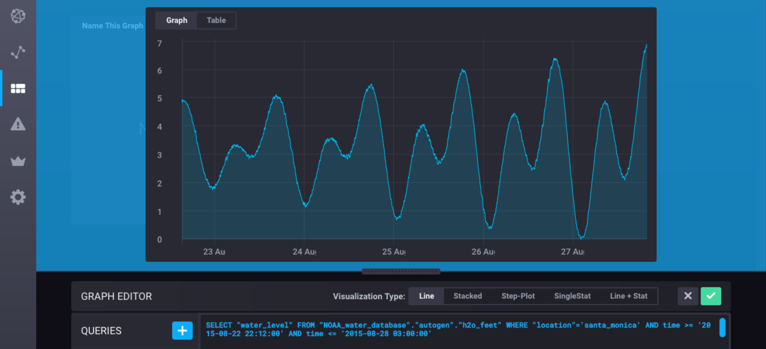
Step 1: Match the Trends of the Raw Data
Write a GROUP BY time() query that matches the general trends of the raw water_level data.
Here, we use the FIRST() function:
SELECT FIRST("water_level") FROM "NOAA_water_database"."autogen"."h2o_feet" WHERE "location"='santa_monica' and time >= '2015-08-22 22:12:00' and time <= '2015-08-28 03:00:00' GROUP BY time(379m,348m)In the GROUP BY time() clause, the first argument (379m) matches
the length of time that occurs between each peak and trough in the water_level data.
The second argument (348m) is the
offset interval.
The offset interval alters the default GROUP BY time() boundaries to
match the time range of the raw data.
The blue line shows the results of the query:

Step 2: Determine the Seasonal Pattern
Identify the seasonal pattern in the data using the information from the query in step 1.
Focusing on the blue line in the graph below, the pattern in the water_level data repeats about every 25 hours and 15 minutes.
There are four data points per season, so 4 is the seasonal pattern argument.

Step 3: Apply the HOLT_WINTERS() function
Add the Holt-Winters function to the query.
Here, we use HOLT_WINTERS_WITH_FIT() to view both the fitted values and the predicted values:
SELECT HOLT_WINTERS_WITH_FIT(FIRST("water_level"),10,4) FROM "NOAA_water_database"."autogen"."h2o_feet" WHERE "location"='santa_monica' AND time >= '2015-08-22 22:12:00' AND time <= '2015-08-28 03:00:00' GROUP BY time(379m,348m)In the HOLT_WINTERS_WITH_FIT() function, the first argument (10) requests 10 predicted field values.
Each predicted point is 379m apart, the same interval as the first argument in the GROUP BY time() clause.
The second argument in the HOLT_WINTERS_WITH_FIT() function (4) is the seasonal pattern that we determined in the previous step.
The blue line shows the results of the query:
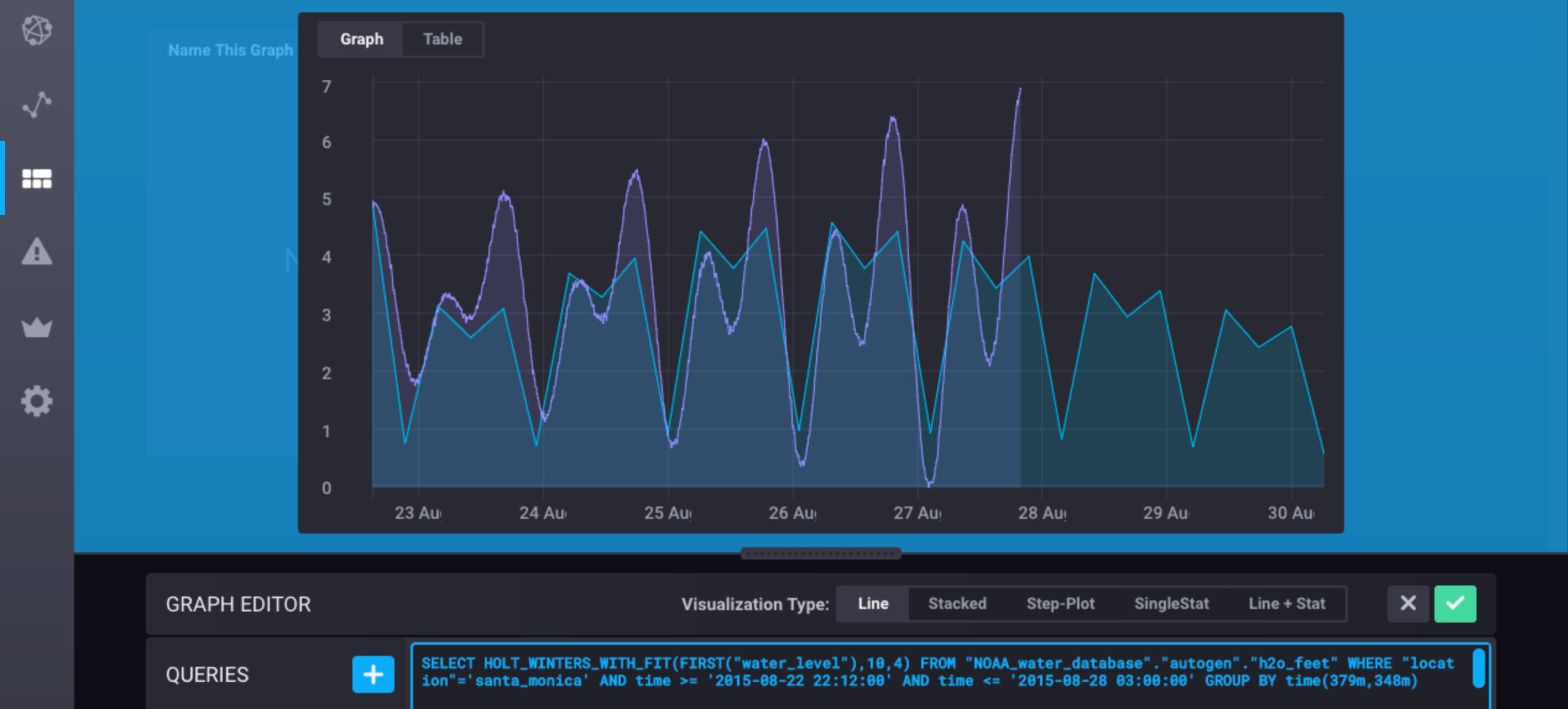
Common Issues with HOLT_WINTERS()
HOLT_WINTERS() and receiving fewer than N points
In some cases, users may receive fewer predicted points than
requested by the N parameter.
That behavior occurs when the math becomes unstable and cannot forecast more
points.
It implies that either HOLT_WINTERS() is not suited for the dataset or that
the seasonal adjustment parameter is invalid and is confusing the algorithm.
Technical Analysis
The following technical analysis functions apply widely used algorithms to your data. While they are primarily used in the world of finance and investing, they have application in other industries and use cases as well.
CHANDE_MOMENTUM_OSCILLATOR()
EXPONENTIAL_MOVING_AVERAGE()
DOUBLE_EXPONENTIAL_MOVING_AVERAGE()
KAUFMANS_EFFICIENCY_RATIO()
KAUFMANS_ADAPTIVE_MOVING_AVERAGE()
TRIPLE_EXPONENTIAL_MOVING_AVERAGE()
TRIPLE_EXPONENTIAL_DERIVATIVE()
RELATIVE_STRENGTH_INDEX()
Arguments
Along with a field key, technical analysis function accept the following arguments:
PERIOD
Required, integer, min=1
The sample size of the algorithm.
This is essentially the number of historical samples which have any significant
effect on the output of the algorithm.
E.G. 2 means the current point and the point before it.
The algorithm uses an exponential decay rate to determine the weight of a historical point,
generally known as the alpha (α). The PERIOD controls the decay rate.
NOTE: Older points can still have an impact.
HOLD_PERIOD
integer, min=-1
How many samples the algorithm needs before it will start emitting results.
The default of -1 means the value is based on the algorithm, the PERIOD,
and the WARMUP_TYPE, but is a value in which the algorithm can emit meaningful results.
Default Hold Periods:
For most of the available technical analysis, the default HOLD_PERIOD is
determined by which technical analysis algorithm you’re using and the WARMUP_TYPE
| Algorithm \ Warmup Type | simple | exponential | none |
|---|---|---|---|
| EXPONENTIAL_MOVING_AVERAGE | PERIOD - 1 | PERIOD - 1 | n/a |
| DOUBLE_EXPONENTIAL_MOVING_AVERAGE | ( PERIOD - 1 ) * 2 | PERIOD - 1 | n/a |
| TRIPLE_EXPONENTIAL_MOVING_AVERAGE | ( PERIOD - 1 ) * 3 | PERIOD - 1 | n/a |
| TRIPLE_EXPONENTIAL_DERIVATIVE | ( PERIOD - 1 ) * 3 + 1 | PERIOD | n/a |
| RELATIVE_STRENGTH_INDEX | PERIOD | PERIOD | n/a |
| CHANDE_MOMENTUM_OSCILLATOR | PERIOD | PERIOD | PERIOD - 1 |
Kaufman Algorithm Default Hold Periods:
| Algorithm | Default Hold Period |
|---|---|
| KAUFMANS_EFFICIENCY_RATIO() | PERIOD |
| KAUFMANS_ADAPTIVE_MOVING_AVERAGE() | PERIOD |
WARMUP_TYPE
default=‘exponential’
This controls how the algorithm initializes itself for the first PERIOD samples.
It is essentially the duration for which it has an incomplete sample set.
simple
Simple moving average (SMA) of the first PERIOD samples.
This is the method used by ta-lib.
exponential
Exponential moving average (EMA) with scaling alpha (α).
This basically uses an EMA with PERIOD=1 for the first point, PERIOD=2
for the second point, etc., until algorithm has consumed PERIOD number of points.
As the algorithm immediately starts using an EMA, when this method is used and
HOLD_PERIOD is unspecified or -1, the algorithm may start emitting points
after a much smaller sample size than with simple.
none
The algorithm does not perform any smoothing at all.
This is the method used by ta-lib.
When this method is used and HOLD_PERIOD is unspecified, HOLD_PERIOD
defaults to PERIOD - 1.
The
nonewarmup type is only available with theCHANDE_MOMENTUM_OSCILLATOR()function.
CHANDE_MOMENTUM_OSCILLATOR()
The Chande Momentum Oscillator (CMO) is a technical momentum indicator developed by Tushar Chande. The CMO indicator is created by calculating the difference between the sum of all recent higher data points and the sum of all recent lower data points, then dividing the result by the sum of all data movement over a given time period. The result is multiplied by 100 to give the -100 to +100 range. Source
Basic syntax
CHANDE_MOMENTUM_OSCILLATOR([ * | <field_key> | /regular_expression/ ], <period>[, <hold_period>, [warmup_type]])Available Arguments:
period
hold_period (Optional)
warmup_type (Optional)
CHANDE_MOMENTUM_OSCILLATOR(field_key, 2)
Returns the field values associated with the field key
processed using the Chande Momentum Oscillator algorithm with a 2-value period
and the default hold period and warmup type.
CHANDE_MOMENTUM_OSCILLATOR(field_key, 10, 9, 'none')
Returns the field values associated with the field key
processed using the Chande Momentum Oscillator algorithm with a 10-value period
a 9-value hold period, and the none warmup type.
CHANDE_MOMENTUM_OSCILLATOR(MEAN(<field_key>), 2) ... GROUP BY time(1d)
Returns the mean of field values associated with the field key
processed using the Chande Momentum Oscillator algorithm with a 2-value period
and the default hold period and warmup type.
Note: When aggregating data with a
GROUP BYclause, you must include an aggregate function in your call to theCHANDE_MOMENTUM_OSCILLATOR()function.
CHANDE_MOMENTUM_OSCILLATOR(/regular_expression/, 2)
Returns the field values associated with each field key that matches the regular expression
processed using the Chande Momentum Oscillator algorithm with a 2-value period
and the default hold period and warmup type.
CHANDE_MOMENTUM_OSCILLATOR(*, 2)
Returns the field values associated with each field key in the measurement
processed using the Chande Momentum Oscillator algorithm with a 2-value period
and the default hold period and warmup type.
CHANDE_MOMENTUM_OSCILLATOR() supports int64 and float64 field value data types.
The basic syntax supports GROUP BY clauses that group by tags but not GROUP BY clauses that group by time.
See the Advanced Syntax section for how to use CHANDE_MOMENTUM_OSCILLATOR() with a GROUP BY time() clause.
EXPONENTIAL_MOVING_AVERAGE()
An exponential moving average (EMA) is a type of moving average that is similar to a simple moving average, except that more weight is given to the latest data. It’s also known as the “exponentially weighted moving average.” This type of moving average reacts faster to recent data changes than a simple moving average.
Basic syntax
EXPONENTIAL_MOVING_AVERAGE([ * | <field_key> | /regular_expression/ ], <period>[, <hold_period)[, <warmup_type]])Available Arguments:
period
hold_period (Optional)
warmup_type (Optional)
EXPONENTIAL_MOVING_AVERAGE(field_key, 2)
Returns the field values associated with the field key
processed using the Exponential Moving Average algorithm with a 2-value period
and the default hold period and warmup type.
EXPONENTIAL_MOVING_AVERAGE(field_key, 10, 9, 'exponential')
Returns the field values associated with the field key
processed using the Exponential Moving Average algorithm with a 10-value period
a 9-value hold period, and the exponential warmup type.
EXPONENTIAL_MOVING_AVERAGE(MEAN(<field_key>), 2) ... GROUP BY time(1d)
Returns the mean of field values associated with the field key
processed using the Exponential Moving Average algorithm with a 2-value period
and the default hold period and warmup type.
Note: When aggregating data with a
GROUP BYclause, you must include an aggregate function in your call to theEXPONENTIAL_MOVING_AVERAGE()function.
EXPONENTIAL_MOVING_AVERAGE(/regular_expression/, 2)
Returns the field values associated with each field key that matches the regular expression
processed using the Exponential Moving Average algorithm with a 2-value period
and the default hold period and warmup type.
EXPONENTIAL_MOVING_AVERAGE(*, 2)
Returns the field values associated with each field key in the measurement
processed using the Exponential Moving Average algorithm with a 2-value period
and the default hold period and warmup type.
EXPONENTIAL_MOVING_AVERAGE() supports int64 and float64 field value data types.
The basic syntax supports GROUP BY clauses that group by tags but not GROUP BY clauses that group by time.
See the Advanced Syntax section for how to use EXPONENTIAL_MOVING_AVERAGE() with a GROUP BY time() clause.
DOUBLE_EXPONENTIAL_MOVING_AVERAGE()
The Double Exponential Moving Average (DEMA) attempts to remove the inherent lag associated to Moving Averages by placing more weight on recent values. The name suggests this is achieved by applying a double exponential smoothing which is not the case. The name double comes from the fact that the value of an EMA is doubled. To keep it in line with the actual data and to remove the lag, the value “EMA of EMA” is subtracted from the previously doubled EMA.
Basic syntax
DOUBLE_EXPONENTIAL_MOVING_AVERAGE([ * | <field_key> | /regular_expression/ ], <period>[, <hold_period)[, <warmup_type]])Available Arguments:
period
hold_period (Optional)
warmup_type (Optional)
DOUBLE_EXPONENTIAL_MOVING_AVERAGE(field_key, 2)
Returns the field values associated with the field key
processed using the Double Exponential Moving Average algorithm with a 2-value period
and the default hold period and warmup type.
DOUBLE_EXPONENTIAL_MOVING_AVERAGE(field_key, 10, 9, 'exponential')
Returns the field values associated with the field key
processed using the Double Exponential Moving Average algorithm with a 10-value period
a 9-value hold period, and the exponential warmup type.
DOUBLE_EXPONENTIAL_MOVING_AVERAGE(MEAN(<field_key>), 2) ... GROUP BY time(1d)
Returns the mean of field values associated with the field key
processed using the Double Exponential Moving Average algorithm with a 2-value period
and the default hold period and warmup type.
Note: When aggregating data with a
GROUP BYclause, you must include an aggregate function in your call to theDOUBLE_EXPONENTIAL_MOVING_AVERAGE()function.
DOUBLE_EXPONENTIAL_MOVING_AVERAGE(/regular_expression/, 2)
Returns the field values associated with each field key that matches the regular expression
processed using the Double Exponential Moving Average algorithm with a 2-value period
and the default hold period and warmup type.
DOUBLE_EXPONENTIAL_MOVING_AVERAGE(*, 2)
Returns the field values associated with each field key in the measurement
processed using the Double Exponential Moving Average algorithm with a 2-value period
and the default hold period and warmup type.
DOUBLE_EXPONENTIAL_MOVING_AVERAGE() supports int64 and float64 field value data types.
The basic syntax supports GROUP BY clauses that group by tags but not GROUP BY clauses that group by time.
See the Advanced Syntax section for how to use DOUBLE_EXPONENTIAL_MOVING_AVERAGE() with a GROUP BY time() clause.
KAUFMANS_EFFICIENCY_RATIO()
Kaufman’s Efficiency Ration, or simply “Efficiency Ratio” (ER), is calculated by dividing the data change over a period by the absolute sum of the data movements that occurred to achieve that change. The resulting ratio ranges between 0 and 1 with higher values representing a more efficient or trending market.
The ER is very similar to the Chande Momentum Oscillator (CMO). The difference is that the CMO takes market direction into account, but if you take the absolute CMO and divide by 100, you you get the Efficiency Ratio.
Basic syntax
KAUFMANS_EFFICIENCY_RATIO([ * | <field_key> | /regular_expression/ ], <period>[, <hold_period>])Available Arguments:
period
hold_period (Optional)
KAUFMANS_EFFICIENCY_RATIO(field_key, 2)
Returns the field values associated with the field key
processed using the Efficiency Index algorithm with a 2-value period
and the default hold period and warmup type.
KAUFMANS_EFFICIENCY_RATIO(field_key, 10, 10)
Returns the field values associated with the field key
processed using the Efficiency Index algorithm with a 10-value period and
a 10-value hold period.
KAUFMANS_EFFICIENCY_RATIO(MEAN(<field_key>), 2) ... GROUP BY time(1d)
Returns the mean of field values associated with the field key
processed using the Efficiency Index algorithm with a 2-value period
and the default hold period.
Note: When aggregating data with a
GROUP BYclause, you must include an aggregate function in your call to theKAUFMANS_EFFICIENCY_RATIO()function.
KAUFMANS_EFFICIENCY_RATIO(/regular_expression/, 2)
Returns the field values associated with each field key that matches the regular expression
processed using the Efficiency Index algorithm with a 2-value period
and the default hold period and warmup type.
KAUFMANS_EFFICIENCY_RATIO(*, 2)
Returns the field values associated with each field key in the measurement
processed using the Efficiency Index algorithm with a 2-value period
and the default hold period and warmup type.
KAUFMANS_EFFICIENCY_RATIO() supports int64 and float64 field value data types.
The basic syntax supports GROUP BY clauses that group by tags but not GROUP BY clauses that group by time.
See the Advanced Syntax section for how to use KAUFMANS_EFFICIENCY_RATIO() with a GROUP BY time() clause.
KAUFMANS_ADAPTIVE_MOVING_AVERAGE()
Kaufman’s Adaptive Moving Average (KAMA) is a moving average designed to account for sample noise or volatility. KAMA will closely follow data points when the data swings are relatively small and noise is low. KAMA will adjust when the data swings widen and follow data from a greater distance. This trend-following indicator can be used to identify the overall trend, time turning points and filter data movements.
Basic syntax
KAUFMANS_ADAPTIVE_MOVING_AVERAGE([ * | <field_key> | /regular_expression/ ], <period>[, <hold_period>])Available Arguments:
period
hold_period (Optional)
KAUFMANS_ADAPTIVE_MOVING_AVERAGE(field_key, 2)
Returns the field values associated with the field key
processed using the Kaufman Adaptive Moving Average algorithm with a 2-value period
and the default hold period and warmup type.
KAUFMANS_ADAPTIVE_MOVING_AVERAGE(field_key, 10, 10)
Returns the field values associated with the field key
processed using the Kaufman Adaptive Moving Average algorithm with a 10-value period
and a 10-value hold period.
KAUFMANS_ADAPTIVE_MOVING_AVERAGE(MEAN(<field_key>), 2) ... GROUP BY time(1d)
Returns the mean of field values associated with the field key
processed using the Kaufman Adaptive Moving Average algorithm with a 2-value period
and the default hold period.
Note: When aggregating data with a
GROUP BYclause, you must include an aggregate function in your call to theKAUFMANS_ADAPTIVE_MOVING_AVERAGE()function.
KAUFMANS_ADAPTIVE_MOVING_AVERAGE(/regular_expression/, 2)
Returns the field values associated with each field key that matches the regular expression
processed using the Kaufman Adaptive Moving Average algorithm with a 2-value period
and the default hold period and warmup type.
KAUFMANS_ADAPTIVE_MOVING_AVERAGE(*, 2)
Returns the field values associated with each field key in the measurement
processed using the Kaufman Adaptive Moving Average algorithm with a 2-value period
and the default hold period and warmup type.
KAUFMANS_ADAPTIVE_MOVING_AVERAGE() supports int64 and float64 field value data types.
The basic syntax supports GROUP BY clauses that group by tags but not GROUP BY clauses that group by time.
See the Advanced Syntax section for how to use KAUFMANS_ADAPTIVE_MOVING_AVERAGE() with a GROUP BY time() clause.
TRIPLE_EXPONENTIAL_MOVING_AVERAGE()
The triple exponential moving average (TEMA) was developed to filter out volatility from conventional moving averages. While the name implies that it’s a triple exponential smoothing, it’s actually a composite of a single exponential moving average, a double exponential moving average, and a triple exponential moving average.
Basic syntax
TRIPLE_EXPONENTIAL_MOVING_AVERAGE([ * | <field_key> | /regular_expression/ ], <period>[, <hold_period)[, <warmup_type]])Available Arguments:
period
hold_period (Optional)
warmup_type (Optional)
TRIPLE_EXPONENTIAL_MOVING_AVERAGE(field_key, 2)
Returns the field values associated with the field key
processed using the Triple Exponential Moving Average algorithm with a 2-value period
and the default hold period and warmup type.
TRIPLE_EXPONENTIAL_MOVING_AVERAGE(field_key, 10, 9, 'exponential')
Returns the field values associated with the field key
processed using the Triple Exponential Moving Average algorithm with a 10-value period
a 9-value hold period, and the exponential warmup type.
TRIPLE_EXPONENTIAL_MOVING_AVERAGE(MEAN(<field_key>), 2) ... GROUP BY time(1d)
Returns the mean of field values associated with the field key
processed using the Triple Exponential Moving Average algorithm with a 2-value period
and the default hold period and warmup type.
Note: When aggregating data with a
GROUP BYclause, you must include an aggregate function in your call to theTRIPLE_EXPONENTIAL_MOVING_AVERAGE()function.
TRIPLE_EXPONENTIAL_MOVING_AVERAGE(/regular_expression/, 2)
Returns the field values associated with each field key that matches the regular expression
processed using the Triple Exponential Moving Average algorithm with a 2-value period
and the default hold period and warmup type.
TRIPLE_EXPONENTIAL_MOVING_AVERAGE(*, 2)
Returns the field values associated with each field key in the measurement
processed using the Triple Exponential Moving Average algorithm with a 2-value period
and the default hold period and warmup type.
TRIPLE_EXPONENTIAL_MOVING_AVERAGE() supports int64 and float64 field value data types.
The basic syntax supports GROUP BY clauses that group by tags but not GROUP BY clauses that group by time.
See the Advanced Syntax section for how to use TRIPLE_EXPONENTIAL_MOVING_AVERAGE() with a GROUP BY time() clause.
TRIPLE_EXPONENTIAL_DERIVATIVE()
The triple exponential derivative indicator, commonly referred to as “TRIX,” is an oscillator used to identify oversold and overbought markets, and can also be used as a momentum indicator. TRIX calculates a triple exponential moving average of the log of the data input over the period of time. The previous value is subtracted from the previous value. This prevents cycles that are shorter than the defined period from being considered by the indicator.
Like many oscillators, TRIX oscillates around a zero line. When used as an oscillator, a positive value indicates an overbought market while a negative value indicates an oversold market. When used as a momentum indicator, a positive value suggests momentum is increasing while a negative value suggests momentum is decreasing. Many analysts believe that when the TRIX crosses above the zero line it gives a buy signal, and when it closes below the zero line, it gives a sell signal.
Basic syntax
TRIPLE_EXPONENTIAL_DERIVATIVE([ * | <field_key> | /regular_expression/ ], <period>[, <hold_period)[, <warmup_type]])Available Arguments:
period
hold_period (Optional)
warmup_type (Optional)
TRIPLE_EXPONENTIAL_DERIVATIVE(field_key, 2)
Returns the field values associated with the field key
processed using the Triple Exponential Derivative algorithm with a 2-value period
and the default hold period and warmup type.
TRIPLE_EXPONENTIAL_DERIVATIVE(field_key, 10, 10, 'exponential')
Returns the field values associated with the field key
processed using the Triple Exponential Derivative algorithm with a 10-value period,
a 10-value hold period, and the exponential warmup type.
TRIPLE_EXPONENTIAL_DERIVATIVE(MEAN(<field_key>), 2) ... GROUP BY time(1d)
Returns the mean of field values associated with the field key
processed using the Triple Exponential Derivative algorithm with a 2-value period
and the default hold period and warmup type.
Note: When aggregating data with a
GROUP BYclause, you must include an aggregate function in your call to theTRIPLE_EXPONENTIAL_DERIVATIVE()function.
TRIPLE_EXPONENTIAL_DERIVATIVE(/regular_expression/, 2)
Returns the field values associated with each field key that matches the regular expression
processed using the Triple Exponential Derivative algorithm with a 2-value period
and the default hold period and warmup type.
TRIPLE_EXPONENTIAL_DERIVATIVE(*, 2)
Returns the field values associated with each field key in the measurement
processed using the Triple Exponential Derivative algorithm with a 2-value period
and the default hold period and warmup type.
TRIPLE_EXPONENTIAL_DERIVATIVE() supports int64 and float64 field value data types.
The basic syntax supports GROUP BY clauses that group by tags but not GROUP BY clauses that group by time.
See the Advanced Syntax section for how to use TRIPLE_EXPONENTIAL_DERIVATIVE() with a GROUP BY time() clause.
RELATIVE_STRENGTH_INDEX()
The relative strength index (RSI) is a momentum indicator that compares the magnitude of recent increases and decreases over a specified time period to measure speed and change of data movements.
Basic syntax
RELATIVE_STRENGTH_INDEX([ * | <field_key> | /regular_expression/ ], <period>[, <hold_period)[, <warmup_type]])Available Arguments:
period
hold_period (Optional)
warmup_type (Optional)
RELATIVE_STRENGTH_INDEX(field_key, 2)
Returns the field values associated with the field key
processed using the Relative Strength Index algorithm with a 2-value period
and the default hold period and warmup type.
RELATIVE_STRENGTH_INDEX(field_key, 10, 10, 'exponential')
Returns the field values associated with the field key
processed using the Relative Strength Index algorithm with a 10-value period,
a 10-value hold period, and the exponential warmup type.
RELATIVE_STRENGTH_INDEX(MEAN(<field_key>), 2) ... GROUP BY time(1d)
Returns the mean of field values associated with the field key
processed using the Relative Strength Index algorithm with a 2-value period
and the default hold period and warmup type.
Note: When aggregating data with a
GROUP BYclause, you must include an aggregate function in your call to theRELATIVE_STRENGTH_INDEX()function.
RELATIVE_STRENGTH_INDEX(/regular_expression/, 2)
Returns the field values associated with each field key that matches the regular expression
processed using the Relative Strength Index algorithm with a 2-value period
and the default hold period and warmup type.
RELATIVE_STRENGTH_INDEX(*, 2)
Returns the field values associated with each field key in the measurement
processed using the Relative Strength Index algorithm with a 2-value period
and the default hold period and warmup type.
RELATIVE_STRENGTH_INDEX() supports int64 and float64 field value data types.
The basic syntax supports GROUP BY clauses that group by tags but not GROUP BY clauses that group by time.
See the Advanced Syntax section for how to use RELATIVE_STRENGTH_INDEX() with a GROUP BY time() clause.
Other
Sample Data
The data used in this document are available for download on the Sample Data page.
General Syntax for Functions
Specify Multiple Functions in the SELECT Clause
Syntax
SELECT <function>(),<function>() FROM_clause [...]Separate multiple functions in one SELECT statement with a comma (,).
The syntax applies to all InfluxQL functions except TOP() and BOTTOM().
The SELECT clause does not support specifying TOP() or BOTTOM() with another function.
Examples
Calculate the mean and median field values in one query
> SELECT MEAN("water_level"),MEDIAN("water_level") FROM "h2o_feet"
name: h2o_feet
time mean median
---- ---- ------
1970-01-01T00:00:00Z 4.442107025822522 4.124The query returns the average and median field values in the water_level field key.
Calculate the mode of two fields in one query
> SELECT MODE("water_level"),MODE("level description") FROM "h2o_feet"
name: h2o_feet
time mode mode_1
---- ---- ------
1970-01-01T00:00:00Z 2.69 between 3 and 6 feetThe query returns the mode field values for the water_level field key and for the level description field key.
The water_level mode is in the mode column and the level description mode is in the mode_1 column.
The system can’t return more than one column with the same name so it renames the second mode column to mode_1.
See Rename the Output Field Key for how to configure the output column headers.
Calculate the minimum and maximum field values in one query
> SELECT MIN("water_level"), MAX("water_level") [...]
name: h2o_feet
time min max
---- --- ---
1970-01-01T00:00:00Z -0.61 9.964The query returns the minimum and maximum field values in the water_level field key.
Notice that the query returns 1970-01-01T00:00:00Z, the InfluxDB equivalent to a null timestamp, as the timestamp value.
MIN() and MAX() are selector functions; when a selector function is the only function in the SELECT clause, it returns a specific timestamp.
Because MIN() and MAX() return two different timestamps (see below), the system overrides those timestamps with the null timestamp equivalent.
> SELECT MIN("water_level") FROM "h2o_feet"
name: h2o_feet
time min
---- ---
2015-08-29T14:30:00Z -0.61 <--- Timestamp 1
> SELECT MAX("water_level") FROM "h2o_feet"
name: h2o_feet
time max
---- ---
2015-08-29T07:24:00Z 9.964 <--- Timestamp 2Rename the Output Field Key
Syntax
SELECT <function>() AS <field_key> [...]By default, functions return results under a field key that matches the function name.
Include an AS clause to specify the name of the output field key.
Examples
Specify the output field key
> SELECT MEAN("water_level") AS "dream_name" FROM "h2o_feet"
name: h2o_feet
time dream_name
---- ----------
1970-01-01T00:00:00Z 4.442107025822522The query returns the average field value of the water_level field key and renames the output field key to dream_name.
Without the AS clause, the query returns mean as the output field key:
> SELECT MEAN("water_level") FROM "h2o_feet"
name: h2o_feet
time mean
---- ----
1970-01-01T00:00:00Z 4.442107025822522Specify the output field key for multiple functions
> SELECT MEDIAN("water_level") AS "med_wat",MODE("water_level") AS "mode_wat" FROM "h2o_feet"
name: h2o_feet
time med_wat mode_wat
---- ------- --------
1970-01-01T00:00:00Z 4.124 2.69The query returns the median and mode field values for the water_level field key and renames the output field keys to med_wat and mode_wat.
Without the AS clauses, the query returns median and mode as the output field keys:
> SELECT MEDIAN("water_level"),MODE("water_level") FROM "h2o_feet"
name: h2o_feet
time median mode
---- ------ ----
1970-01-01T00:00:00Z 4.124 2.69Change the Values Reported for Intervals with no Data
By default, queries with an InfluxQL function and a GROUP BY time() clause report null values for intervals with no data.
Include fill() at the end of the GROUP BY clause to change that value.
See Data Exploration for a complete discussion of fill().
Common Issues with Functions
The following sections describe frequent sources of confusion with all functions, aggregation functions, and selector functions. See the function-specific documentation for common issues with individual functions:
All Functions
Nesting functions
Some InfluxQL functions support nesting in the SELECT clause:
COUNT()withDISTINCT()CUMULATIVE_SUM()DERIVATIVE()DIFFERENCE()ELAPSED()MOVING_AVERAGE()NON_NEGATIVE_DERIVATIVE()HOLT_WINTERS()andHOLT_WINTERS_WITH_FIT()
For other functions, use InfluxQL’s subqueries to nest functions in the FROM clause.
See the Data Exploration page more on using subqueries.
Querying time ranges after now()
Most SELECT statements have a default time range between 1677-09-21 00:12:43.145224194 and 2262-04-11T23:47:16.854775806Z UTC.
For SELECT statements with an InfluxQL function and a GROUP BY time() clause, the default time
range is between 1677-09-21 00:12:43.145224194 UTC and now().
To query data with timestamps that occur after now(), SELECT statements with
an InfluxQL function and a GROUP BY time() clause must provide an alternative upper bound in the
WHERE clause.
See the Frequently Asked Questions page for an example.
Aggregation Functions
Understanding the returned timestamp
A query with an aggregation function and no time range in the WHERE clause returns epoch 0 (1970-01-01T00:00:00Z) as the timestamp.
InfluxDB uses epoch 0 as the null timestamp equivalent.
A query with an aggregate function that includes a time range in the WHERE clause returns the lower time bound as the timestamp.
Examples
Use an aggregate function without a specified time range
> SELECT SUM("water_level") FROM "h2o_feet"
name: h2o_feet
time sum
---- ---
1970-01-01T00:00:00Z 67777.66900000004The query returns the InfluxDB equivalent of a null timestamp (epoch 0: 1970-01-01T00:00:00Z) as the timestamp.
SUM() aggregates points across several timestamps and has no single timestamp to return.
Use an aggregate function with a specified time range
> SELECT SUM("water_level") FROM "h2o_feet" WHERE time >= '2015-08-18T00:00:00Z'
name: h2o_feet
time sum
---- ---
2015-08-18T00:00:00Z 67777.66900000004The query returns the lower time bound (WHERE time >= '2015-08-18T00:00:00Z') as the timestamp.
Use an aggregate function with a specified time range and a GROUP BY time() clause
> SELECT SUM("water_level") FROM "h2o_feet" WHERE time >= '2015-08-18T00:00:00Z' AND time <= '2015-08-18T00:18:00Z' GROUP BY time(12m)
name: h2o_feet
time sum
---- ---
2015-08-18T00:00:00Z 20.305
2015-08-18T00:12:00Z 19.802999999999997The query returns the lower time bound for each GROUP BY time() interval as the timestamps.
Mixing aggregation functions with non-aggregates
Aggregation functions do not support specifying standalone field keys or tag keys in the SELECT clause.
Aggregation functions return a single calculated value and there is no obvious single value to return for any unaggregated fields or tags.
Including a standalone field key or tag key with an aggregation function in the SELECT clause returns an error:
> SELECT SUM("water_level"),"location" FROM "h2o_feet"
ERR: error parsing query: mixing aggregate and non-aggregate queries is not supportedGetting slightly different results
For some aggregation functions, executing the same function on the same set of float64 points may yield slightly different results. InfluxDB does not sort points before it applies the aggregation function; that behavior can cause small discrepancies in the query results.
Selector Functions
Understanding the returned timestamp
The timestamps returned by selector functions depend on the number of functions in the query and on the other clauses in the query:
A query with a single selector function, a single field key argument, and no GROUP BY time() clause returns the timestamp for the point that appears in the raw data.
A query with a single selector function, multiple field key arguments, and no GROUP BY time() clause returns the timestamp for the point that appears in the raw data or the InfluxDB equivalent of a null timestamp (epoch 0: 1970-01-01T00:00:00Z).
A query with more than one function and no time range in the WHERE clause returns the InfluxDB equivalent of a null timestamp (epoch 0: 1970-01-01T00:00:00Z).
A query with more than one function and a time range in the WHERE clause returns the lower time bound as the timestamp.
A query with a selector function and a GROUP BY time() clause returns the lower time bound for each GROUP BY time() interval.
Note that the SAMPLE() function behaves differently from other selector functions when paired with the GROUP BY time() clause.
See Common Issues with SAMPLE() for more information.
Examples
Use a single selector function with a single field key and without a specified time range
> SELECT MAX("water_level") FROM "h2o_feet"
name: h2o_feet
time max
---- ---
2015-08-29T07:24:00Z 9.964
> SELECT MAX("water_level") FROM "h2o_feet" WHERE time >= '2015-08-18T00:00:00Z'
name: h2o_feet
time max
---- ---
2015-08-29T07:24:00Z 9.964The queries return the timestamp for the maximum point that appears in the raw data.
Use a single selector function with multiple field keys and without a specified time range
> SELECT FIRST(*) FROM "h2o_feet"
name: h2o_feet
time first_level description first_water_level
---- ----------------------- -----------------
1970-01-01T00:00:00Z between 6 and 9 feet 8.12
> SELECT MAX(*) FROM "h2o_feet"
name: h2o_feet
time max_water_level
---- ---------------
2015-08-29T07:24:00Z 9.964The first query returns the InfluxDB equivalent of a null timestamp (epoch 0: 1970-01-01T00:00:00Z) as the timestamp.
FIRST(*) returns two timestamps (one for each field key in the h2o_feet measurement) so the system overrides those timestamps with the null timestamp equivalent.
The second query returns the timestamp for the maximum point that appears in the raw data.
MAX(*) returns one timestamp (the h2o-feet measurement has only one numerical field) so the system does not overwrite the original timestamp.
Use a selector function with another function and without a specified time range
> SELECT MAX("water_level"),MIN("water_level") FROM "h2o_feet"
name: h2o_feet
time max min
---- --- ---
1970-01-01T00:00:00Z 9.964 -0.61The query returns the InfluxDB equivalent of a null timestamp (epoch 0: 1970-01-01T00:00:00Z) as the timestamp.
The MAX() and MIN() functions return different timestamps so the system has no single timestamp to return.
Use a selector function with another function and with a specified time range
> SELECT MAX("water_level"),MIN("water_level") FROM "h2o_feet" WHERE time >= '2015-08-18T00:00:00Z'
name: h2o_feet
time max min
---- --- ---
2015-08-18T00:00:00Z 9.964 -0.61The query returns the lower time bound (WHERE time >= '2015-08-18T00:00:00Z') as the timestamp.
Use a selector function with a GROUP BY time() clause
> SELECT MAX("water_level") FROM "h2o_feet" WHERE time >= '2015-08-18T00:00:00Z' AND time <= '2015-08-18T00:18:00Z' GROUP BY time(12m)
name: h2o_feet
time max
---- ---
2015-08-18T00:00:00Z 8.12
2015-08-18T00:12:00Z 7.887The query returns the lower time bound for each GROUP BY time() interval as the timestamp.
Was this page helpful?
Thank you for your feedback!
Support and feedback
Thank you for being part of our community! We welcome and encourage your feedback and bug reports for InfluxDB OSS v1 and this documentation. To find support, use the following resources:
Customers with an annual or support contract can contact InfluxData Support.